![]()
Probabilistic and continuous modelling :
Gaussian process learning
![]()
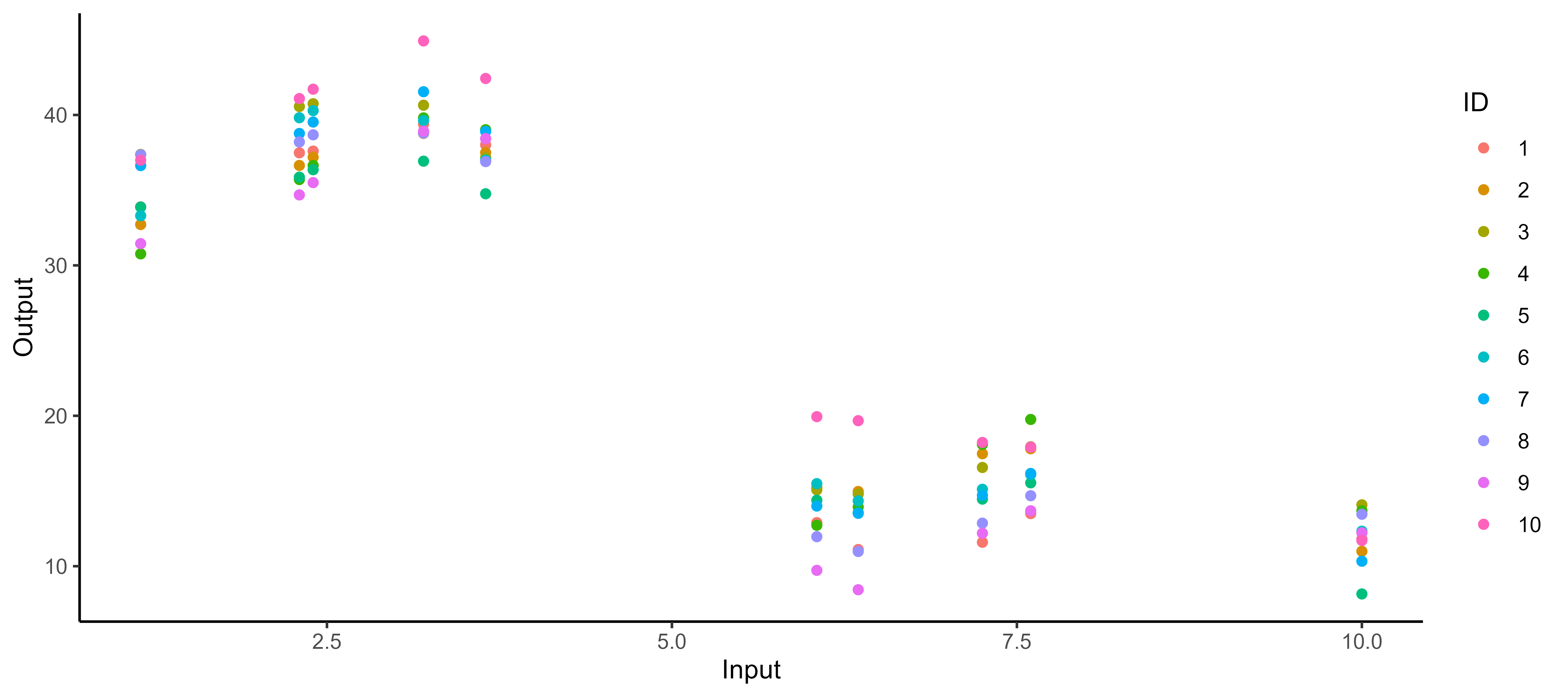
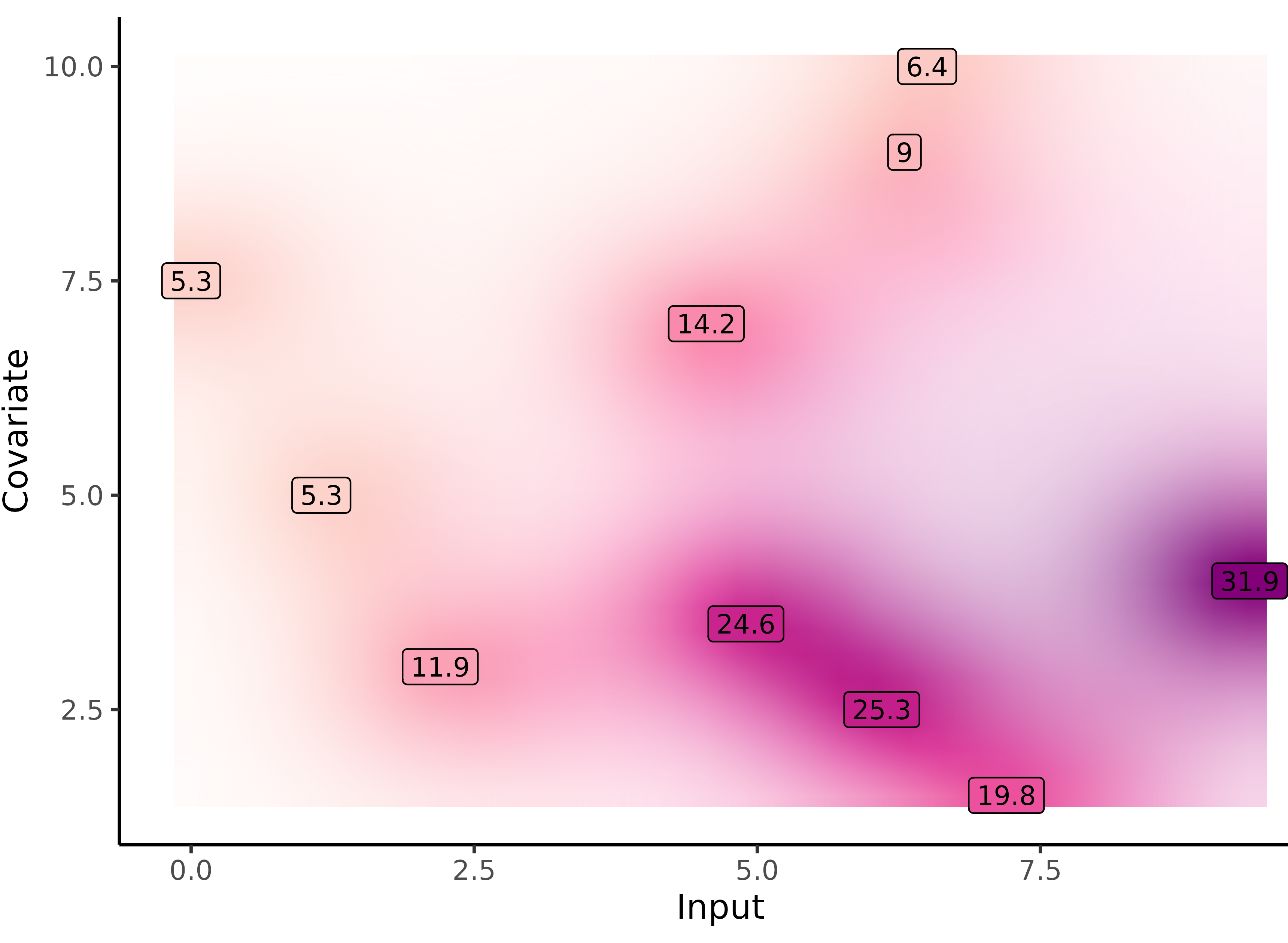
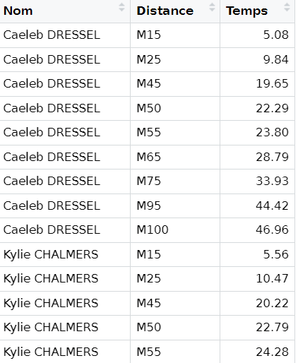
Motivation: can you spot the differences?
![]()
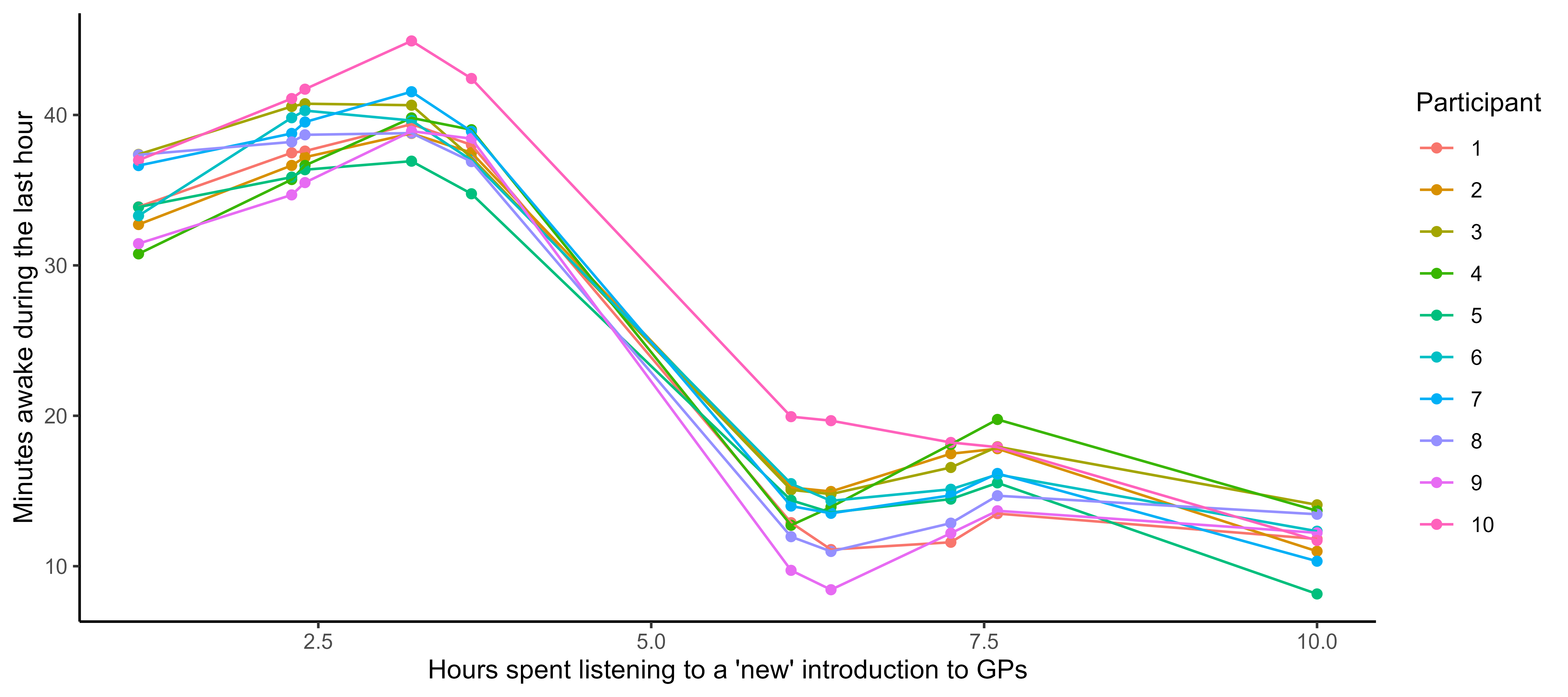
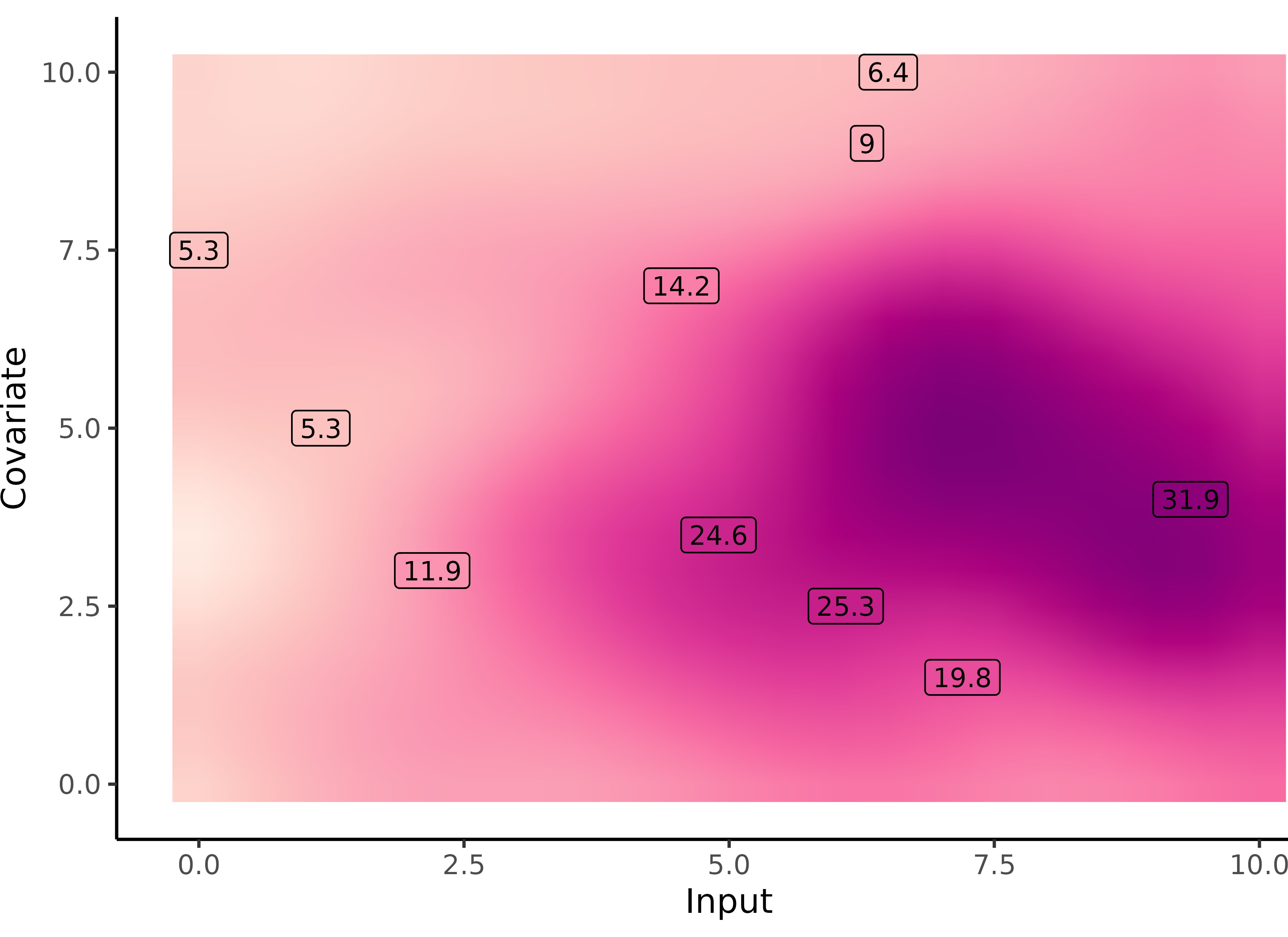
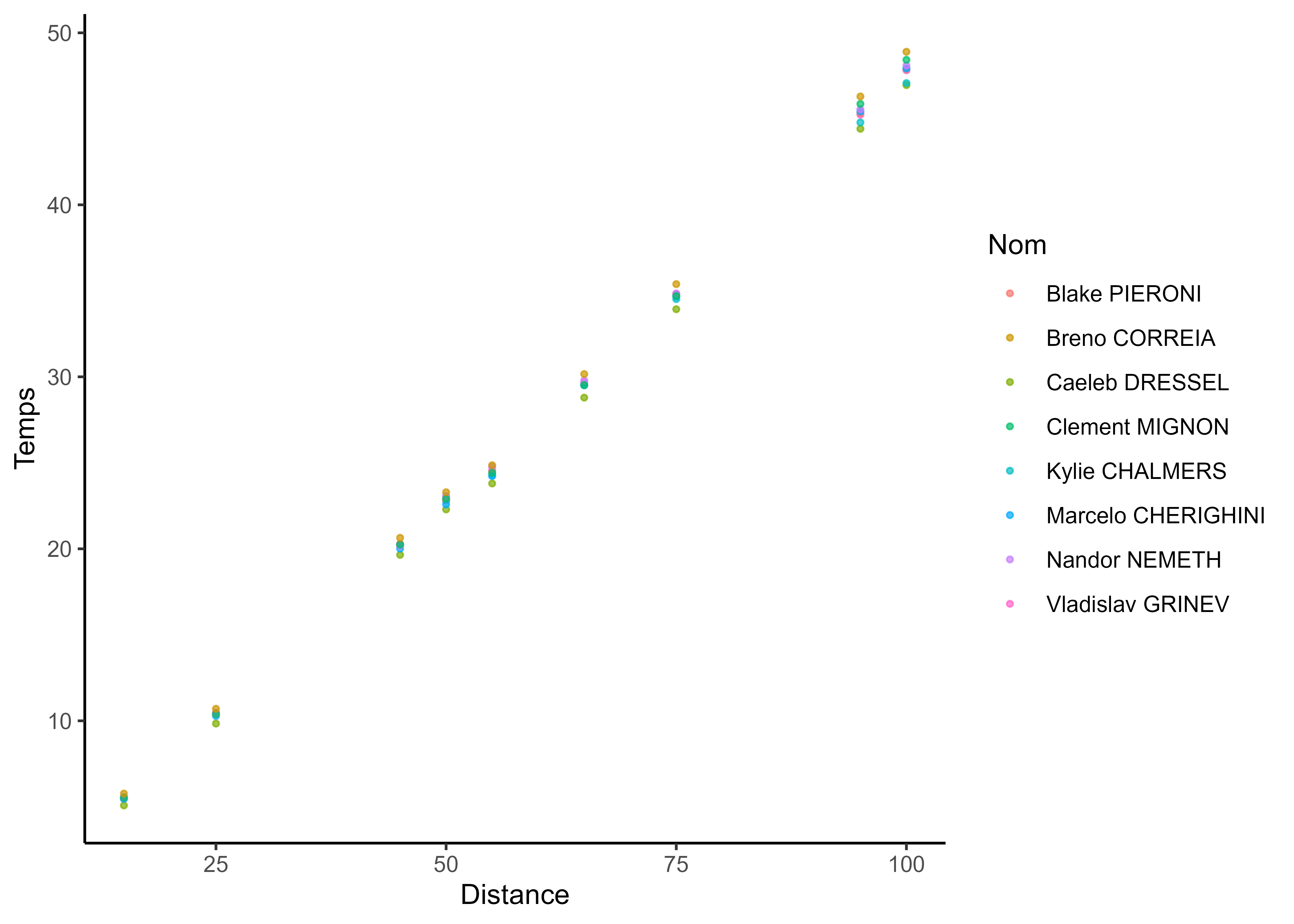
Motivation: can you spot the differences?
![]()
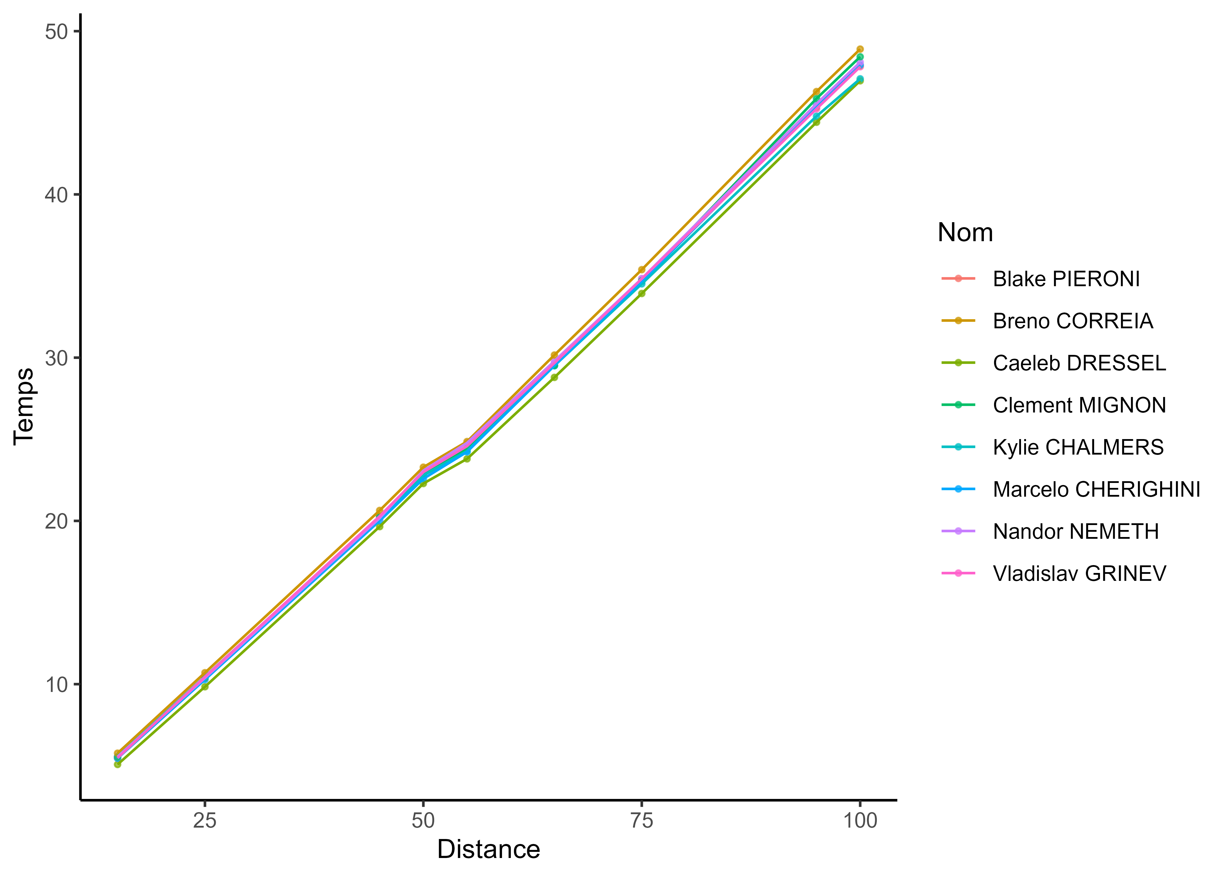
Functional/continuous data is all about smoothness and tidiness
![]()
![]()
Functional/continuous data is all about smoothness and tidiness
![]()
![]()
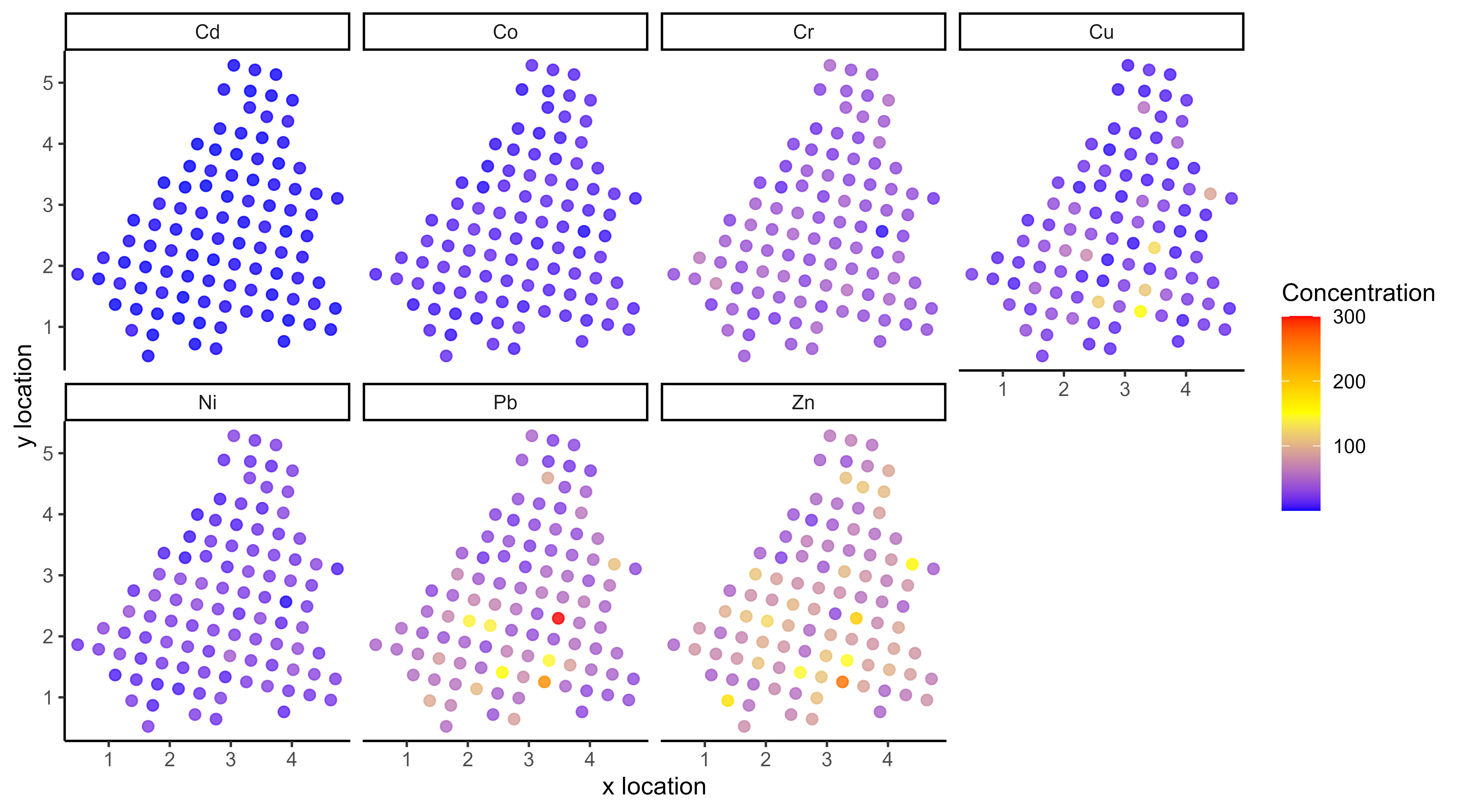
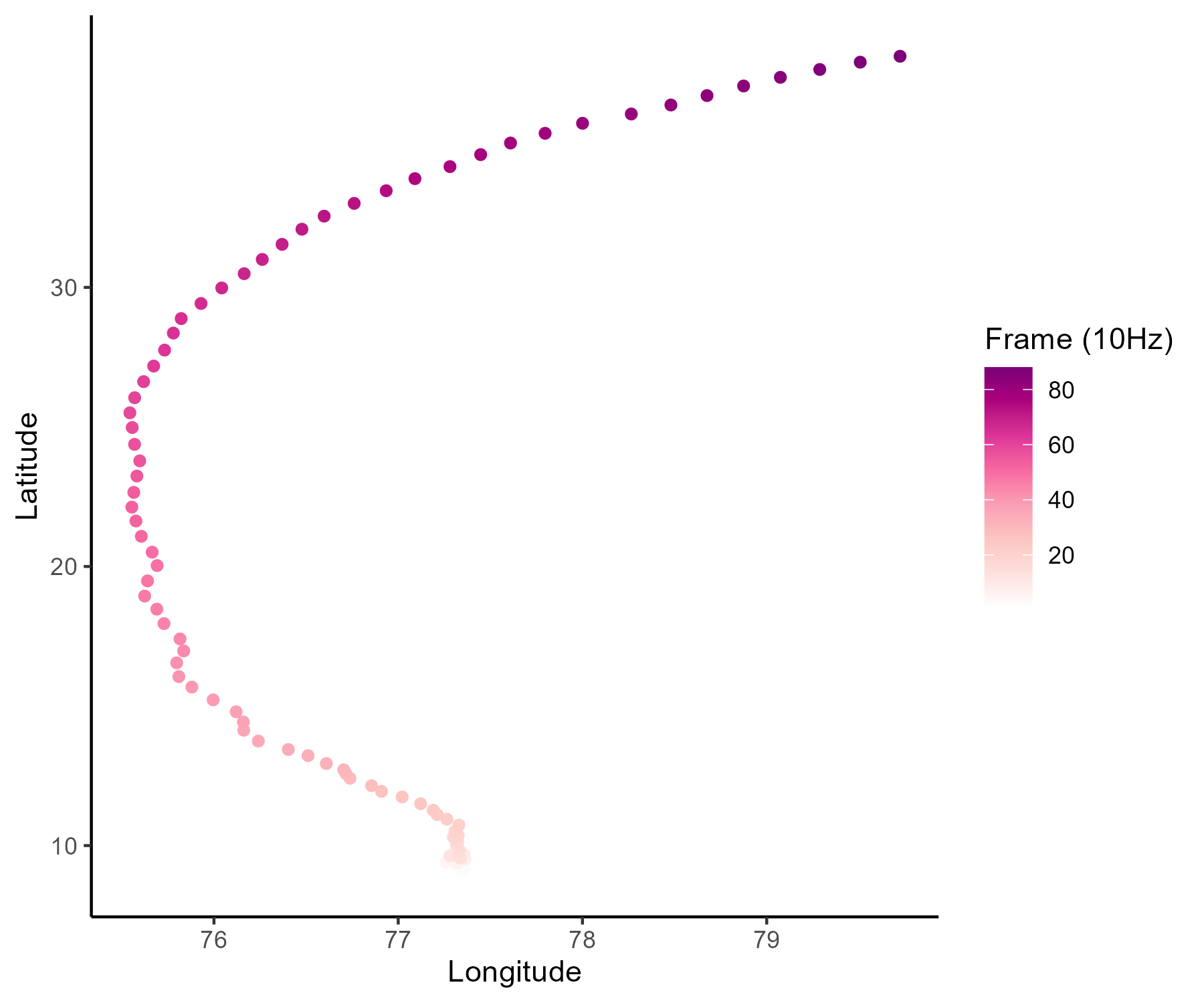
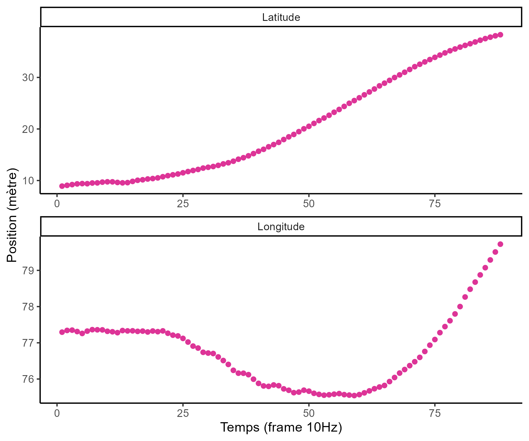
Time, space and continua
![]()
![]()
Supervised learning as a functional regression problem
\[y = \color{orange}{f}(x) + \epsilon\]
where:
- \(x\) is the input variable (typically time, location, any continuum),
- \(y\) is the output variable (typically performance measurements),
- \(\epsilon\) is the noise, a random error term,
- \(\color{orange}{f}\) is a random function encoding the relationship between input and output data.
All supervised learning problems require to retrieve the most reliable function \(\color{orange}{f}\), using observed data \(\{(x_1, y_1), \dots, (x_n, y_n) \}\), to perform predictions when observing new input data \(x_{n+1}\).
Learning the simplest of functions : linear regression
In the simplest (though really common in practice) case of linear regression, we assume that:
\[\color{orange}{f}(x) = a x + b\]
Finding the best function \(\color{orange}{f}\) reduces to compute optimal parameters \(a\) and \(b\) from our dataset.
![]()
Probabilistic learning
A probabilistic modelling approach consists in defining a prior distribution over possible functions \(\color{orange}{f}\), and use data to update our beliefs to derive a posterior distribution over functions.
This approach has several advantages:
- It allows to quantify uncertainty in predictions and can lead to more robust models
- It provides a principled way to incorporate prior knowledge
- It can be used for both regression and classification tasks
- It provides a framework for model comparison and selection
As discussed ealier, Bayes’ theorem is the cornerstone of probabilistic learning:
\[p(\color{orange}{f} \mid \text{data}) \propto p(\text{data} \mid \color{orange}{f}) \times p(\color{orange}{f})\]
Choosing a prior over functions
Several choices are possible to define a prior distribution over functions \(\color{orange}{f}\):
- Parametric approaches: e.g., Bayesian linear regression assumes a Gaussian prior over parameters \(a\) and \(b\).
- Non-parametric approaches: e.g., Gaussian processes define a prior directly over the space of functions.
In this course, we focus on Gaussian processes (GPs), a powerful and flexible non-parametric approach to model distributions over functions.
Before diving into GPs, let’s briefly review multivariate Gaussian distributions, which are the building blocks of GPs.
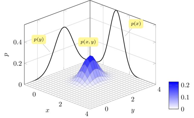
Multivariate Gaussian distributions
The probability density function of a multivariate Gaussian distribution is: \[p(x) = \frac{1}{(2\pi)^{d/2} |\Sigma|^{1/2}} \exp\left(-\frac{1}{2}(x - \mu)^T \Sigma^{-1} (x - \mu)\right)\] where
- \(x \in \mathbb{R}\) \(^d\) is a random vector,
- \(\mu \in \mathbb{R}^d\) is the mean vector,
- \(\Sigma \in \mathbb{R}^{d \times d}\) is the covariance matrix.
The diagonal of \(\Sigma\) represent variances of each dimension; off-diagonal elements represent covariances across dimensions.
Stability under marginalisation
\[\begin{pmatrix} X_1 \\ X_2 \end{pmatrix} \sim \mathcal{N}\left( \begin{pmatrix} \mu_1 \\ \mu_2 \end{pmatrix}, \begin{pmatrix} \Sigma_{11} & \Sigma_{12} \\ \Sigma_{21} & \Sigma_{22} \end{pmatrix} \right) \implies X_1 \sim \mathcal{N}(\mu_1, \Sigma_{11})\]
![]()
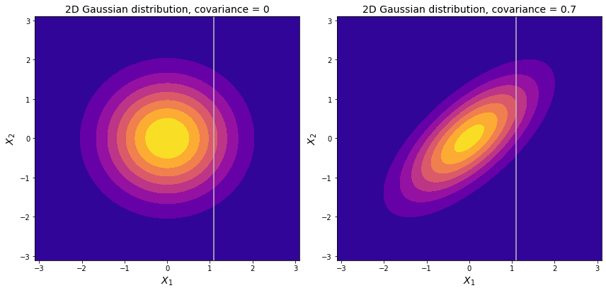
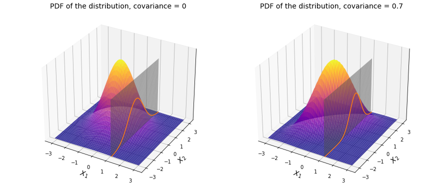
Stability under conditionning
\[\begin{pmatrix} X_1 \\ X_2 \end{pmatrix} \sim \mathcal{N}\left( \begin{pmatrix} \mu_1 \\ \mu_2 \end{pmatrix}, \begin{pmatrix} \Sigma_{11} & \Sigma_{12} \\ \Sigma_{21} & \Sigma_{22} \end{pmatrix} \right) \implies X_1 | X_2 \sim \mathcal{N}(\mu_{1|2}, \Sigma_{1|2})\]
where \[\begin{align*}
\mu_{1|2} &= \mu_1 + \Sigma_{12} \Sigma_{22}^{-1} (X_2 - \mu_2) \\
\Sigma_{1|2} &= \Sigma_{11} - \Sigma_{12} \Sigma_{22}^{-1} \Sigma_{21}
\end{align*}\]
![]()
Stability under conditionning (illustration)
![]()
Stability under conditionning (proof sketch)
\[p(X_1 | X_2) = \frac{p(X_1, X_2)}{p(X_2)}
= \frac{\mathcal{N}\left( \begin{pmatrix} X_1 \\ X_2 \end{pmatrix} | \begin{pmatrix} \mu_1 \\ \mu_2 \end{pmatrix}, \begin{pmatrix} \Sigma_{11} & \Sigma_{12} \\ \Sigma_{21} & \Sigma_{22} \end{pmatrix} \right)}{\mathcal{N}(X_2 | \mu_2, \Sigma_{22})}\]
To derive the conditional distribution, we can follow these steps:
- Write the joint distribution \(p(X_1, X_2)\) and the marginal distribution \(p(X_2)\) using the multivariate Gaussian density formula.
- Combine the exponents from the numerator and denominator.
- Complete the square in the exponent to identify the mean and covariance of the conditional distribution.
Gaussian process: a prior distribution over functions
\[y = \color{orange}{f}(x) + \epsilon\]
No restrictions on \(\color{orange}{f}\) but a prior distribution on a functional space: \(\color{orange}{f} \sim \mathcal{GP}(m(\cdot),C(\cdot,\cdot))\)
We can think of a Gaussian process as the extension to infinity of multivariate Gaussians:
\[p(f_1, f_2, \ldots, f_N, \ldots \mid \mathbf{x})
= \mathcal{N}\left(
\begin{bmatrix}
m(x_1) \\
m(x_2) \\
\vdots \\
m(x_N) \\
\vdots
\end{bmatrix},
\begin{bmatrix}
C(x_1,x_1) & C(x_1,x_2) & \cdots & C(x_1,x_N) & \cdots \\
C(x_2,x_1) & C(x_2,x_2) & \cdots & C(x_2,x_N) & \cdots \\
\vdots & \vdots & \ddots & \vdots & \\
C(x_N,x_1) & C(x_N,x_2) & \cdots & C(x_N,x_N) & \cdots \\
\vdots & \vdots & & \vdots & \ddots
\end{bmatrix}
\right)\]
A GP is like a long cake and each slice is a Gaussian
![]()
Credits: Carl Henrik Ek
A GP is like an infinitely long cake and each slice is a Gaussian
![]()
Credits: Carl Henrik Ek
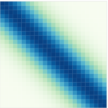
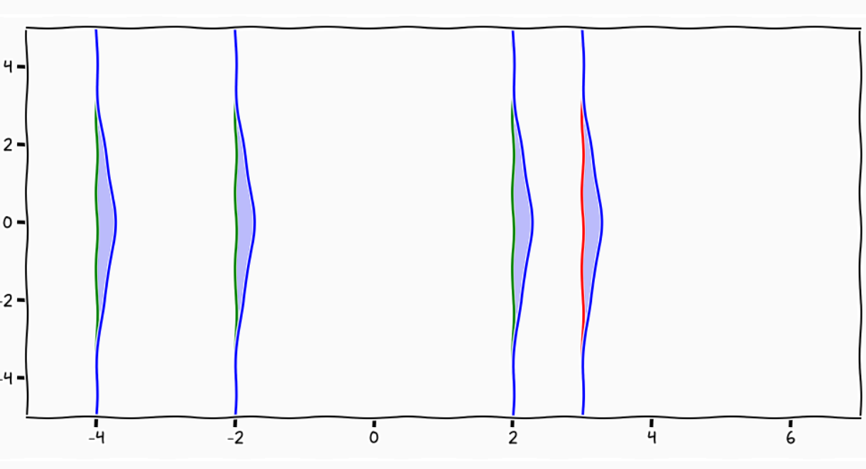
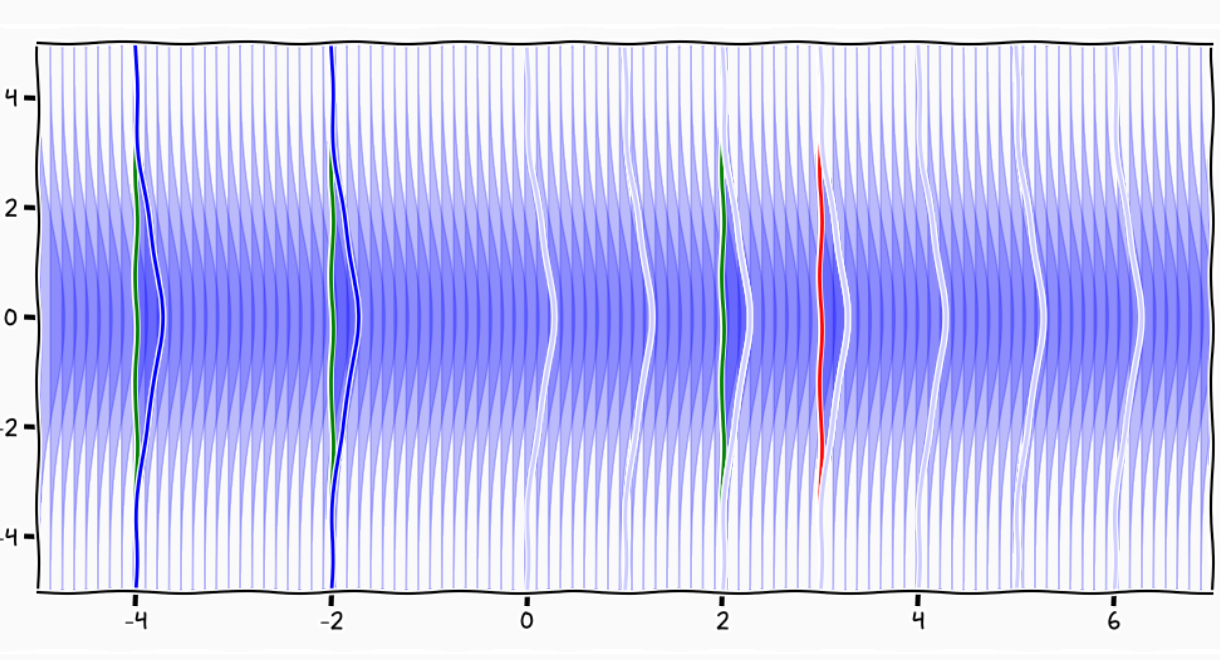
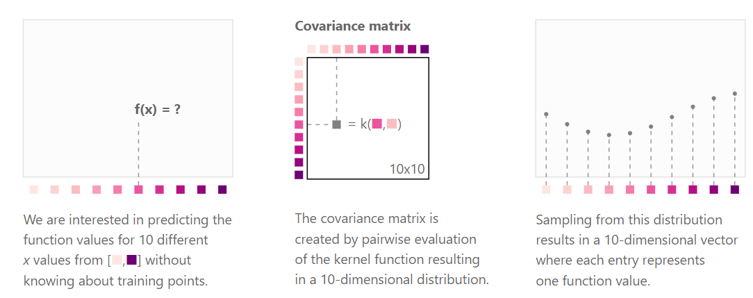
Kernels and covariance functions
Kernels (or covariance functions) \(C(\cdot, \cdot)\) define the covariance structure of functions sampled from a GP. Formally, we fill the covariance matrix \(K\) such that:
\[cov(f(x), f(x^{\prime})) = C(x, x^{\prime}) = \left[C \right]_{x, x^{\prime}}.\]
![]() https://distill.pub/2019/visual-exploration-gaussian-processes/
https://distill.pub/2019/visual-exploration-gaussian-processes/
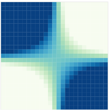
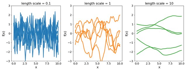
Covariance functions: Squared Exponential kernel
While \(m(\cdot)\) is often assumed to be \(0\), the covariance structure is critical and defined through tailored kernels. For instance, the Squared Exponential (or RBF) kernel is expressed as: \[C_{SE}(x, x^{\prime}) = s^2 \exp \Bigg(-\dfrac{(x - x^{\prime})^2}{2 \ell^2}\Bigg)\]
![]()
![]()
Covariance functions: Periodic kernel
To model phenomenon exhibiting repeting patterns, one can leverage the Periodic kernel: \[C_{perio}(x, x^{\prime}) = s^2 \exp \Bigg(- \dfrac{ 2 \sin^2 \Big(\pi \frac{\mid x - x^{\prime}\mid}{p} \Big)}{\ell^2}\Bigg)\]
![]()
![]()
Covariance functions: Linear kernel
We can even consider linear regression as a particular GP problem, by using the Linear kernel: \[C_{lin}(x, x^{\prime}) = s_a^2 + s_b^2 (x - c)(x^{\prime} - c )\]
![]()
![]()
We can learn optimal values of hyper-parameters from data through maximum likelihood.
Gaussian process regression model
Given observed data \(\mathbf{y} = (y_1, \dots, y_n)^T\) at inputs \(\mathbf{x} = (x_1, \dots, x_n)^T\), we assume:
\[y_i = \color{orange}{f}(x_i) + \epsilon_i, \hspace{1cm} \forall i = 1, \dots, n\]
with
- \(\color{orange}{f} \sim \mathcal{GP}(m(\cdot), C_{\theta}(\cdot, \cdot))\),
- \(\epsilon_i \sim \mathcal{N}(0, \sigma^2)\), independent noise terms.
The vector of observations \(\mathbf{y}\) follows a multivariate Gaussian distribution:
\[\mathbf{y} \sim \mathcal{N}(m(\mathbf{x}), C_{\theta}(\mathbf{x}, \mathbf{x}) + \sigma^2 I)\]
where \(C_{\theta}(\mathbf{x}, \mathbf{x})\) is the covariance matrix evaluated at inputs \(\mathbf{x}\), with hyper-parameters \(\theta\).
Question: Write the proof for this result using the properties of Gaussian distributions.
Proof
\[\begin{align*}
p(\mathbf{y}) &= \int p(\mathbf{y} \mid f) p(f) \ \mathrm{d}f \\
&= \int \mathcal{N}(\mathbf{y}; f(\mathbf{x}), \sigma^2 I) \ \mathcal{N}(f(\mathbf{x}); m(\mathbf{x}), C_{\theta}(\mathbf{x}, \mathbf{x})) \ \mathrm{d}f
\end{align*}\]
Using the property that the convolution of two Gaussians is Gaussian, we can compute its mean:
\[\begin{align*}
\mathbb{E}[\mathbf{y}] &= \int \mathbf{y} \ p(\mathbf{y}) \ \mathrm{d}\mathbf{y} \\
&= \int \mathbf{y} \int p(\mathbf{y} \mid f) p(f) \ \mathrm{d}f \ \mathrm{d}\mathbf{y} \\
&= \int \int \mathbf{y} \ p(\mathbf{y} \mid f) \ \mathrm{d}\mathbf{y} \ p(f) \ \mathrm{d}f \\
&= \int \underbrace{\mathbb{E}_{\mathbf{y} \mid f} \left[\mathbf{y} \right] }_{f(\mathbf{x})} \ p(f) \ \mathrm{d}f \\
&= \mathbb{E}_{f} \left[f(\mathbf{x}) \right] = m(\mathbf{x}).
\end{align*}\]
Proof (continued)
… and second order moment:
\[\begin{align*}
\mathbb{E}[\mathbf{y} \mathbf{y}^T] &= \int \mathbf{y} \mathbf{y}^T \ p(\mathbf{y}) \ \mathrm{d}\mathbf{y} \\
&= \int \int \mathbf{y} \mathbf{y}^T \ p(\mathbf{y} \mid f) \ \mathrm{d}\mathbf{y} \ p(f) \ \mathrm{d}f \\
&= \int \underbrace{\mathbb{E}_{\mathbf{y} \mid f} \left[\mathbf{y} \mathbf{y}^T \right] }_{f(\mathbf{x}) f(\mathbf{x})^T + \sigma^2 I} \ p(f) \ \mathrm{d}f \\
&= \mathbb{E}_{f} \left[f(\mathbf{x}) f(\mathbf{x})^T \right] + \sigma^2 I \\
&= C_{\theta}(\mathbf{x}, \mathbf{x}) + m(\mathbf{x}) m(\mathbf{x})^T + \sigma^2 I.
\end{align*}\]
We can now compute the variance:
\[\begin{align*}
\mathrm{Var}[\mathbf{y}] &= \mathbb{E}[\mathbf{y} \mathbf{y}^T] - \mathbb{E}[\mathbf{y}] \mathbb{E}[\mathbf{y}]^T \\
&= C_{\theta}(\mathbf{x}, \mathbf{x}) + \sigma^2 I.
\end{align*}\]
Optimising hyper-parameters of the kernel
The log-marginal likelihood of observed data \(\mathbf{y}\) given inputs \(\mathbf{x}\) and hyper-parameters \(\theta\) is: \[\log p(\mathbf{y} \mid \mathbf{x}, \theta) = -\frac{1}{2} \mathbf{y}^T (C_{\theta} + \sigma^2 I )^{-1} \mathbf{y} - \frac{1}{2} \log |C_{\theta} + \sigma^2 I| - \frac{n}{2} \log 2\pi.\]
We can optimise hyper-parameters \(\theta\) by maximizing the log-marginal likelihood using gradient-based methods.
![]()
Source: 10.48550/arXiv.2511.12550
Gaussian process prediction: all you need is a posterior
The Gaussian property induces that unobserved points have no influence on inference:
\[ \int \underbrace{p(f_{\color{grey}{obs}}, f_{\color{purple}{mis}})}_{\mathcal{GP}(m, C)} \ \mathrm{d}f_{\color{purple}{mis}} = \underbrace{p(f_{\color{grey}{obs}})}_{\mathcal{N}(m_{\color{grey}{obs}}, C_{\color{grey}{obs}})}\]
This crucial trick allows us to learn function properties from finite sets of observations. More generally, Gaussian processes are closed under conditioning and marginalisation.
\[\begin{bmatrix}
f_{\color{grey}{o}} \\
f_{\color{purple}{m}} \\
\end{bmatrix} \sim \mathcal{N} \left(
\begin{bmatrix}
m_{\color{grey}{o}} \\
m_{\color{purple}{m}} \\
\end{bmatrix},
\begin{pmatrix}
C_{\color{grey}{o, o}} & C_{\color{grey}{o}, \color{purple}{m}} \\
C_{\color{purple}{m}, \color{grey}{o}} & C_{\color{purple}{m, m}}
\end{pmatrix} \right)\]
While marginalisation serves for training, conditioning leads the key GP prediction formula:
\[f_{\color{purple}{m}} \mid f_{\color{grey}{o}} \sim \mathcal{N} \Big(
m_{\color{purple}{m}} + C_{\color{purple}{m}, \color{grey}{o}} C_{\color{grey}{o, o}}^{-1} (f_{\color{grey}{o}} - m_{\color{grey}{o}}), \ \ C_{\color{purple}{m, m}} - C_{\color{purple}{m}, \color{grey}{o}} C_{\color{grey}{o, o}}^{-1} C_{\color{grey}{o}, \color{purple}{m}} \Big)\]
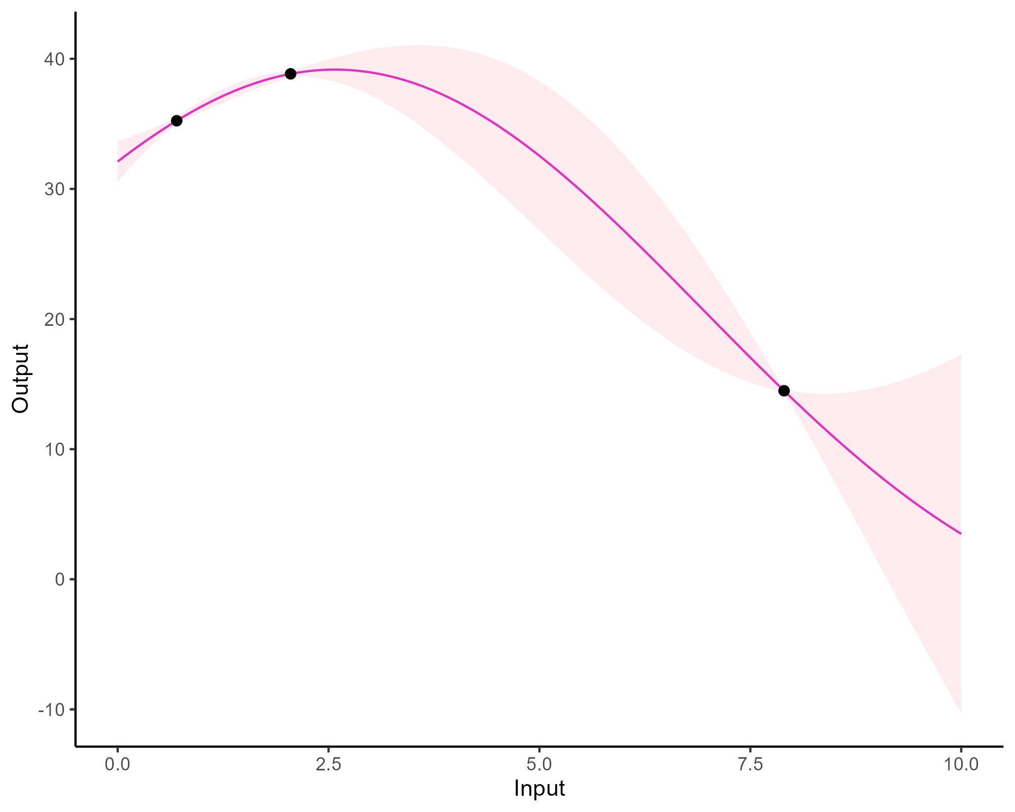
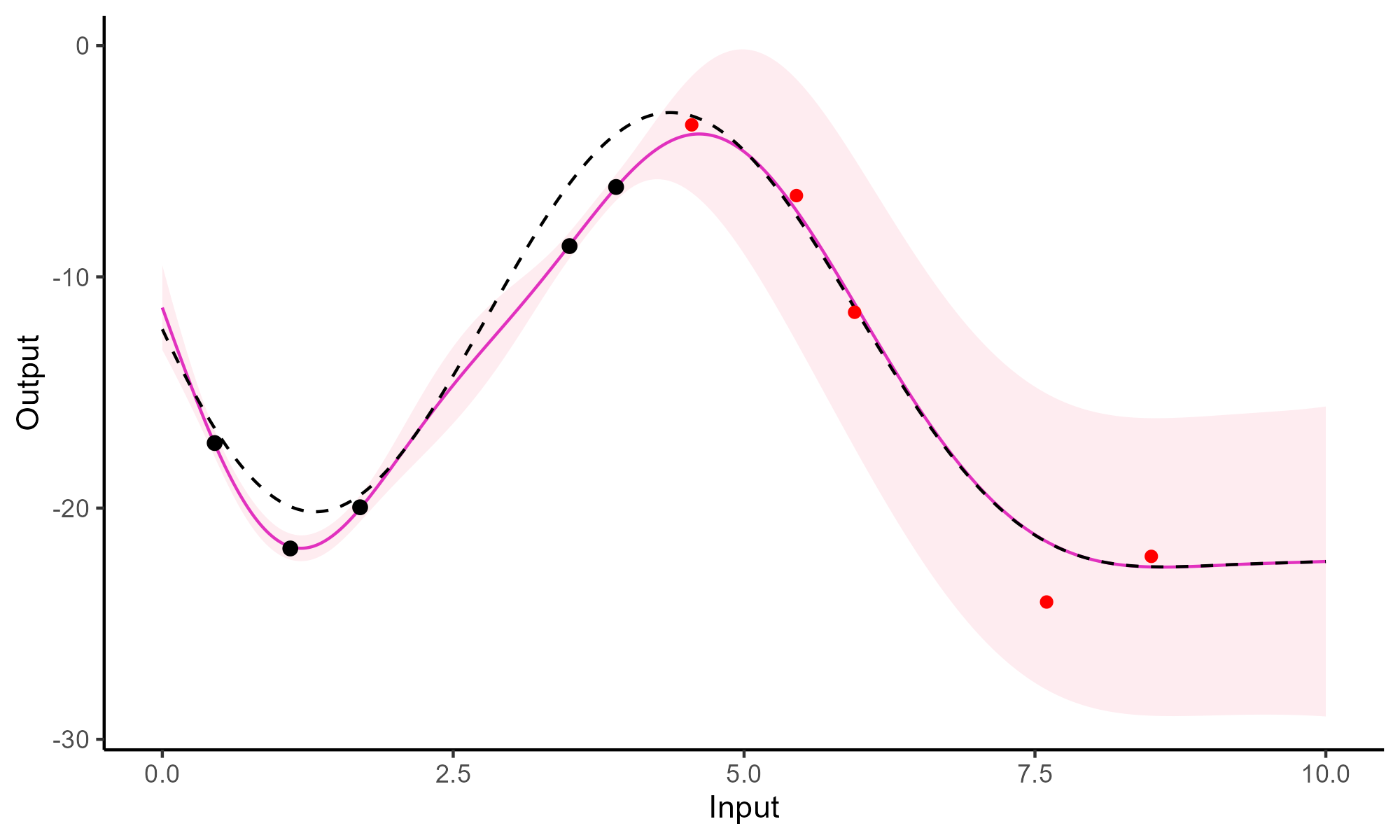
A visual summary of GP regression: prior and optimisation
![]()
![]()
\(f \sim \mathcal{GP}(0, C_{SE}(\cdot, \cdot))\) \(\hat{\theta} = \text{argmax}_{\theta} \log p(\mathbf{y} \mid \mathbf{x}, \theta)\)
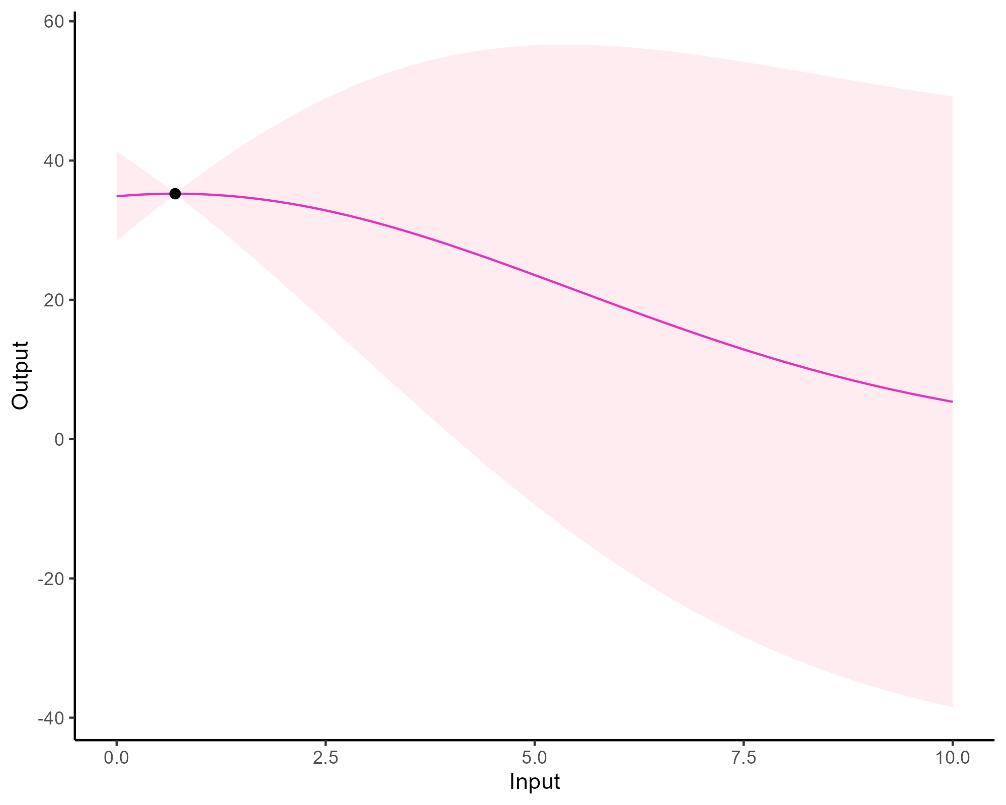
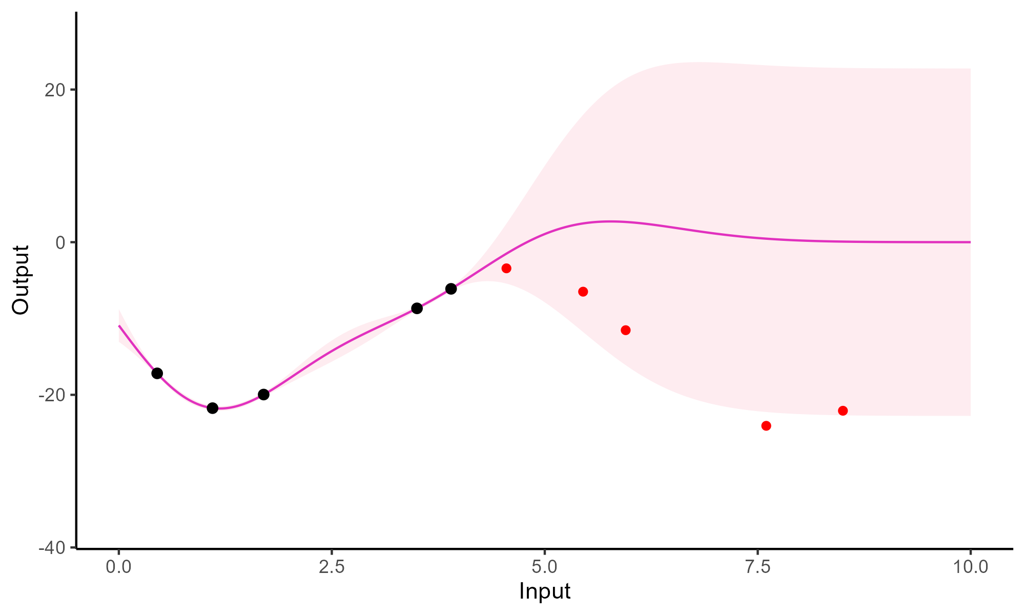
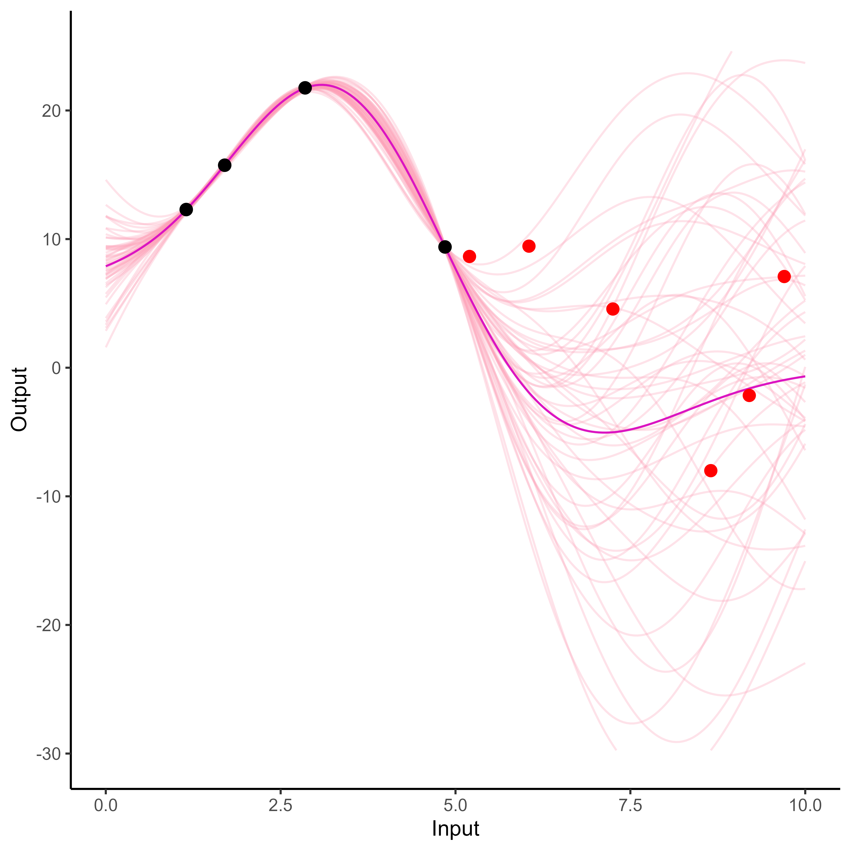
Prediction: updating our knowledge about functions
![]()
![]()
\(f_{\color{purple}{m}} \mid f_{\color{grey}{o}} \sim \mathcal{N} \Big(
m_{\color{purple}{m}} + C_{\color{purple}{m}, \color{grey}{o}} C_{\color{grey}{o, o}}^{-1} (f_{\color{grey}{o}} - m_{\color{grey}{o}}), \ \ C_{\color{purple}{m, m}} - C_{\color{purple}{m}, \color{grey}{o}} C_{\color{grey}{o, o}}^{-1} C_{\color{grey}{o}, \color{purple}{m}} \Big)\)
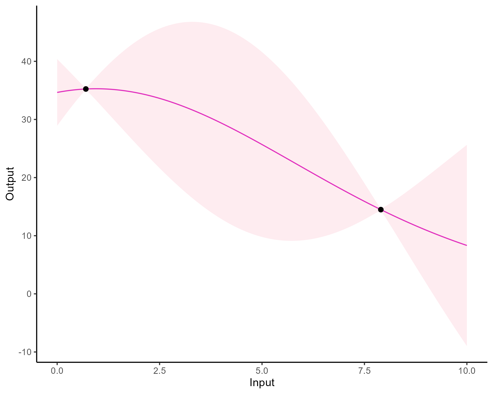
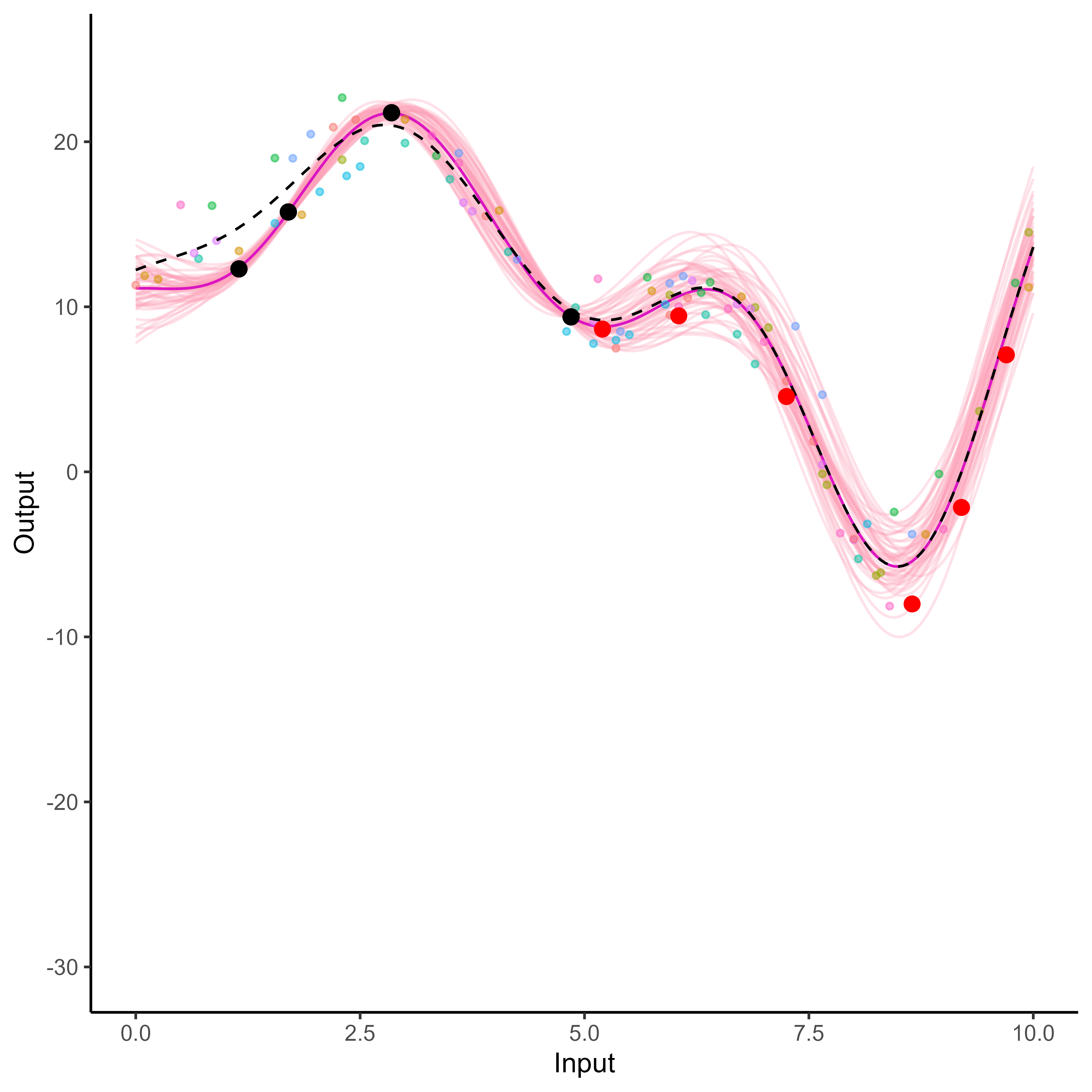
Forecasting with a GP
![]()
Forecasting with a GP
![]()
Multi-Output and Multi-task
Gaussian processes
![]()
It all starts with observations from multiple sources …
![]()
It all starts with observations from multiple sources …
![]()
… but sometimes we are not measuring the same things …
![]()
… among many other difficulties …
![]()
Several classical challenges:
- Irregular measurements (in number of observations and location),
… among many other difficulties …
![]()
Several classical challenges:
- Irregular measurements (in number of observations and location),
- Multiple sources of data (athletes, sensors, …)
… or all of them at once!
![]()
Multi-Task? Multi-Output? What are the maths behind that?
In the previous examples, we saw a variety of situations that naturally lead to the same mathematical formulation of the learning problem:
\[y_s = \color{orange}{f_s}(x_s) + \epsilon_s, \hspace{3cm} \forall s = 1, \dots, S\]
Learn \(\color{orange}{f_s}\), the underlying relationship between \(x_s\) and \(y_s\), for each source of data \(\color{orange}{s}\).
Multi-, in contrast with single-, regression implies that some information can be shared across data sources to improve learning/predictions.
The nature of measurements leads to a more philosophical distinction:
- Multi-Output clearly refers to several variables of interest. An Output is a quantity we aim to infer/predict from Input measurements, and which may be correlated with others.
- Multi-Task implies the existence of an underlying pattern, shared by several tasks or individuals, which can be jointly exploited to build a common model.
Multi-Task Gaussian Processes
\[y_t = \mu_0 + f_t + \epsilon_t, \hspace{3cm} \forall t = 1, \dots, T\]
with:
- \(\mu_0 \sim \mathcal{GP}(m_0, K_{0}),\)
- \(f_t \sim \mathcal{GP}(0, \Sigma_{\theta_t}), \ \perp \!\!\! \perp_t,\)
- \(\epsilon_t \sim \mathcal{GP}(0, \sigma_t^2), \ \perp \!\!\! \perp_t.\)
It follows that:
\[y_t \mid \mu_0 \sim \mathcal{GP}(\mu_0, \Sigma_{\theta_t} + \sigma_t^2 I), \ \perp \!\!\! \perp_t\]
\(\rightarrow\) Unified GP framework with a shared mean process \(\mu_0\), and task-specific process \(f_t\), \(\rightarrow\) Naturaly handles irregular grids of input data.
Goal: Learn the hyper-parameters, (and \(\mu_0\)’s hyper-posterior). Difficulty: The likelihood depends on \(\mu_0\), and tasks are not independent.
Notation and dimensionality
Each task has its specific vector of inputs \(\color{purple}{\textbf{x}_i}\) associated with outputs \(\textbf{y}_i\). The mean process \(\mu_0\) requires to define pooled vectors and additional notation follows:
- \(\textbf{y} = (\textbf{y}_1,\dots, \textbf{y}_i, \dots, \textbf{y}_M)^T,\)
- \(\color{grey}{\textbf{x}} = (\textbf{x}_1,\dots,\textbf{x}_i, \dots, \textbf{x}_M)^T,\)
- \(\textbf{K}_{0}^{\color{grey}{\textbf{x}}}\): covariance matrix from the process \(\mu_0\) evaluated on \(\color{grey}{\textbf{x}},\)
- \(\boldsymbol{\Sigma}_{\theta_t}^{\color{purple}{\textbf{x}_i}}\): covariance matrix from the process \(f_t\) evaluated on \(\color{purple}{\color{purple}{\textbf{x}_i}},\)
- \(\Theta = \{(\theta_t)_i, \sigma_t^2 \}\): the set of hyper-parameters,
- \(\boldsymbol{\Psi}_{\theta_t, \sigma_t^2}^{\color{purple}{\textbf{x}_i}} = \boldsymbol{\Sigma}_{\theta_t}^{\color{purple}{\textbf{x}_i}} + \sigma_t^2 I_{N_i}\).
While GP are infinite-dimensional objects, a tractable inference on a finite set of observations fully determines the overall properties.
EM algorithm
E-step
\[
\begin{align}
p(\mu_0(\color{grey}{\mathbf{x}}) \mid \textbf{y}, \hat{\Theta})
&\propto \mathcal{N}(\mu_0(\color{grey}{\mathbf{x}}); m_0(\color{grey}{\textbf{x}}), \textbf{K}_{0}^{\color{grey}{\textbf{x}}}) \times \prod\limits_{t =1}^T \mathcal{N}(\mathbf{y}_t; \mu_0( \color{purple}{\textbf{x}_i}), \boldsymbol{\Psi}_{\hat{\theta}_i, \hat{\sigma}_i^2}^{\color{purple}{\textbf{x}_i}}) \\
&= \mathcal{N}(\mu_0(\color{grey}{\mathbf{x}}); \hat{m}_0(\color{grey}{\textbf{x}}), \hat{\textbf{K}}^{\color{grey}{\textbf{x}}}),
\end{align}
\]
- \(\hat{\textbf{K}}^{\color{grey}{\textbf{x}}} = ({\textbf{K}_{0}^{\color{grey}{\textbf{x}}}}^{-1} + \sum\limits_{t = 1}^T {\boldsymbol{\Psi}_{\hat{\theta}_i, \hat{\sigma}_i^2}^{\color{purple}{\textbf{x}_i}}}^{-1})^{-1}\)
- \(\hat{m}_0(\color{grey}{\textbf{x}}) = \hat{\textbf{K}}^{\color{grey}{\textbf{x}}}({\textbf{K}_{0}^{\color{grey}{\textbf{x}}}}^{-1} m_0(\color{grey}{\mathbf{x}}) + \sum\limits_{t = 1}^T {\boldsymbol{\Psi}_{\hat{\theta}_i, \hat{\sigma}_i^2}^{\color{purple}{\textbf{x}_i}}}^{-1} \mathbf{y}_t)\).
M-step
\[
\begin{align*}
\hat{\Theta}
&= \underset{\Theta}{\arg\max} \ \ \sum\limits_{t = 1}^{T}\left\{ \log \mathcal{N} \left( \mathbf{y}_t; \hat{m}_0(\color{purple}{\mathbf{x}_t}), \boldsymbol{\Psi}_{\theta_t, \sigma^2}^{\color{purple}{\mathbf{x}_t}} \right) - \dfrac{1}{2} Tr \left( \hat{\mathbf{K}}^{\color{purple}{\mathbf{x}_t}} {\boldsymbol{\Psi}_{\theta_t, \sigma^2}^{\color{purple}{\mathbf{x}_t}}}^{-1} \right) \right\}.
\end{align*}
\]
Covariance structure assumption and computational complexity
Sharing the covariance structures or not offers a compromise between flexibility and parsimony:
- One optimisation problem for \(\theta\), and a shared process for all tasks,
- \(\color{blue}{T}\) distinct optimisation problems for \(\{\theta_t\}_t\), and task-specific processes.
Major interests:
- Both approaches scale linearly with the number of tasks,
- Parallel computing can be used to speed up training.
Overall, the computational complexity is: \[
\mathcal{O}(\color{blue}{T} \times N_t^3 + N^3)
\]
with \(N = \bigcup\limits_{t = 1}^\color{blue}{T} N_t\)
Prediction
For a new task, we observe some data \(y_*(\textbf{x}_*)\). Let us recall:
\[y_* \mid \mu_0 \sim \mathcal{GP}(\mu_0, \boldsymbol{\Psi}_{\theta_*, \sigma_*^2}), \ \perp \!\!\! \perp_t\]
Goals:
- derive a analytical predictive distribution at arbitrary inputs \(\mathbf{x}^{p}\),
- sharing the information from training tasks, stored in the mean process \(\mu_0\).
Difficulties:
- the model is conditionned over \(\mu_0\), a latent, unobserved quantity,
- defining the adequate target distribution is not straightforward,
- working on a new grid of inputs \(\mathbf{x}^{p}_{*}= (\mathbf{x}_{*}, \mathbf{x}^{p})^{\intercal},\) potentially distinct from \(\mathbf{x}.\)
Prediction: the key idea
Defining a multi-task prior distribution by:
- conditioning on training data,
- integrating over \(\mu_0\)’s hyper-posterior distribution.
\[\begin{align}
p(y_* (\textbf{x}_*^{p}) \mid \textbf{y})
&= \int p\left(y_* (\textbf{x}_*^{p}) \mid \textbf{y}, \mu_0(\textbf{x}_*^{p})\right) p(\mu_0 (\textbf{x}_*^{p}) \mid \textbf{y}) \ d \mu_0(\mathbf{x}^{p}_{*}) \\
&= \int \underbrace{ p \left(y_* (\textbf{x}_*^{p}) \mid \mu_0 (\textbf{x}_*^{p}) \right)}_{\mathcal{N}(y_*; \mu_0, \Psi_*)} \ \underbrace{p(\mu_0 (\textbf{x}_*^{p}) \mid \textbf{y})}_{\mathcal{N}(\mu_0; \hat{m}_0, \hat{K})} \ d \mu_0(\mathbf{x}^{p}_{*}) \\
&= \mathcal{N}( \hat{m}_0 (\mathbf{x}^{p}_{*}), \underbrace{\Psi_* + \hat{K}}_{\Gamma})
\end{align}\]
Predictions with Multi-Task GPs
\[p \left( \begin{bmatrix}
y_*(\color{grey}{\mathbf{x}_{*}}) \\
y_*(\color{purple}{\mathbf{x}^{p}}) \\
\end{bmatrix} \mid \textbf{y} \right) = \mathcal{N} \left(
\begin{bmatrix}
y_*(\color{grey}{\mathbf{x}_{*}}) \\
y_*(\color{purple}{\mathbf{x}^{p}}) \\
\end{bmatrix}; \
\begin{bmatrix}
\hat{m}_0(\color{grey}{\mathbf{x}_{*}}) \\
\hat{m}_0(\color{purple}{\mathbf{x}^{p}}) \\
\end{bmatrix},
\begin{pmatrix}
\Gamma_{\color{grey}{**}} & \Gamma_{\color{grey}{*}\color{purple}{p}} \\
\Gamma_{\color{purple}{p}\color{grey}{*}} & \Gamma_{\color{purple}{pp}}
\end{pmatrix} \right)\]
\[p(y_*(\color{purple}{\mathbf{x}^{p}}) \mid y_*(\color{grey}{\mathbf{x}_{*}}), \textbf{y}) = \mathcal{N} \Big( y_*(\color{purple}{\mathbf{x}^{p}}); \ \hat{\mu}_{*}(\color{purple}{\mathbf{x}^{p}}) , \hat{\Gamma}_{\color{purple}{pp}} \Big)\]
with:
- \(\hat{\mu}_{*}(\color{purple}{\mathbf{x}^{p}}) = \hat{m}_0(\color{purple}{\mathbf{x}^{p}}) + \Gamma_{\color{purple}{p}\color{grey}{*}}\Gamma_{\color{grey}{**}}^{-1} (y_*(\color{grey}{\mathbf{x}_{*}}) - \hat{m}_0 (\color{grey}{\mathbf{x}_{*}}))\)
- \(\hat{\Gamma}_{\color{purple}{pp}} = \Gamma_{\color{purple}{pp}} - \Gamma_{\color{purple}{p}\color{grey}{*}}\Gamma_{\color{grey}{**}}^{-1} \Gamma_{\color{grey}{*}\color{purple}{p}}\)
A GIF is worth a thousand words
![]()
A GIF is worth a thousand words
![]()
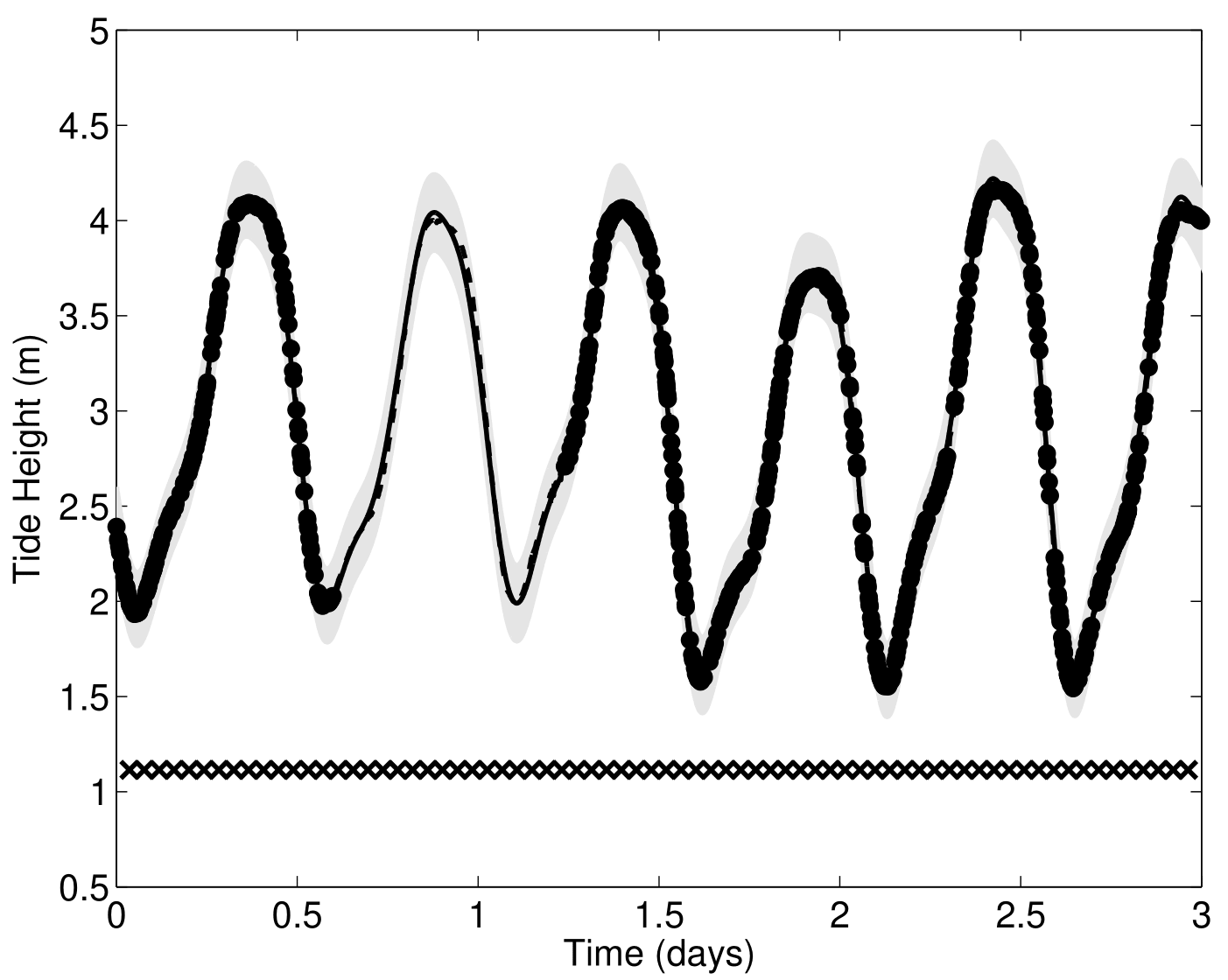
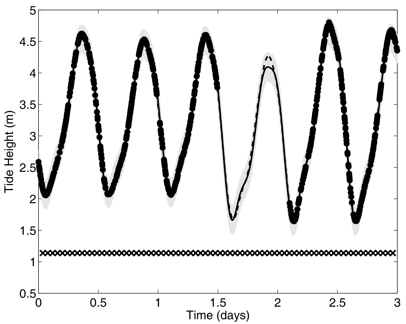
Comparison with single GP regression
![]()
![]()
Yet another comparison with single GP regression but in 2D
![]()
![]()
Multi-Task GPs regression provides more reliable predictions when individual processes are sparsely observed, while greatly reducing the associated uncertainty
Your turn to work again
![]()
Time to fit some Multi-Task GPs!
![]()
![image alt >]()
We will extensively use the MagmaClustR package for modelling functional data with GPs.
Mixture of Gaussian Processes and Clustering
![]()
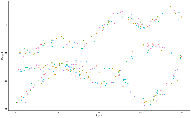
Group patterns in functional data
![]()
Adding some clustering into Multi-Task GPs
A unique underlying mean process might be too restrictive.
\(\rightarrow\) Mixture of multi-task GPs:
\[y_t = \mu_0 + f_t + \epsilon_t, \hspace{3cm} \forall t = 1, \dots, T\]
with:
- \(\color{green}{Z_{t}} \sim \mathcal{M}(1, \color{green}{\boldsymbol{\pi}}), \ \perp \!\!\! \perp_t,\)
- \(\mu_0 \sim \mathcal{GP}(m_0, K_0),\)
- \(f_t \sim \mathcal{GP}(0, \Sigma_{\theta_t}), \ \perp \!\!\! \perp_t,\)
- \(\epsilon_t \sim \mathcal{GP}(0, \sigma_t^2), \ \perp \!\!\! \perp_t.\)
It follows that:
\[y_t \mid \mu_0 \sim \mathcal{GP}(\mu_0, \Psi_t), \ \perp \!\!\! \perp_t\]
Adding some clustering into Multi-Task GPs
A unique underlying mean process might be too restrictive.
\(\rightarrow\) Mixture of multi-task GPs:
\[y_t \mid \{\color{green}{Z_{tk}} = 1 \} = \mu_{\color{green}{k}} + f_t + \epsilon_t, \hspace{3cm} \forall t = 1, \dots, T\]
with:
- \(\color{green}{Z_{t}} \sim \mathcal{M}(1, \color{green}{\boldsymbol{\pi}}), \ \perp \!\!\! \perp_t,\)
- \(\mu_{\color{green}{k}} \sim \mathcal{GP}(m_{\color{green}{k}}, \color{green}{C_{{k}}})\ \perp \!\!\! \perp_{\color{green}{k}},\)
- \(f_t \sim \mathcal{GP}(0, \Sigma_{\theta_t}), \ \perp \!\!\! \perp_t,\)
- \(\epsilon_t \sim \mathcal{GP}(0, \sigma_t^2), \ \perp \!\!\! \perp_t.\)
It follows that:
\[y_t \mid \{ \boldsymbol{\mu} , \color{green}{\boldsymbol{\pi}} \} \sim \sum\limits_{k=1}^K{ \color{green}{\pi_k} \ \mathcal{GP}\Big(\mu_{\color{green}{k}}, \Psi_t^\color{green}{k} \Big)}, \ \perp \!\!\! \perp_t\]
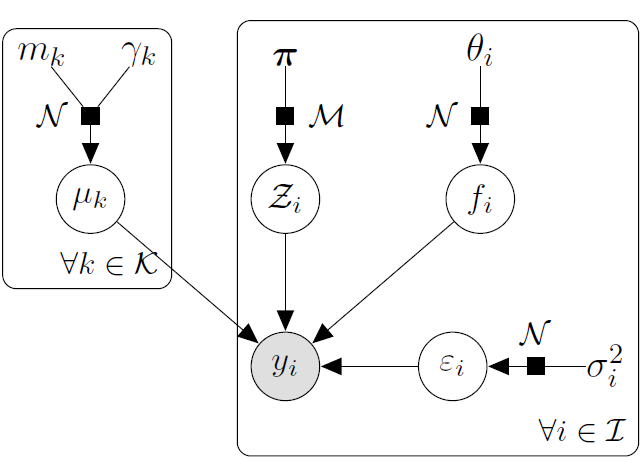
Exercise time
Draw the hierarchical graphical model corresponding to the previous mixture of multi-task GPs, from the model assumptions.
Variational inference : motivation
In the mixture of GPs model, we have two sets of latent variables:
- The cluster-specific mean processes: \( \boldsymbol{\mu} = \{\mu_\color{green}{k}\}_\color{green}{k}\),
- The cluster assignments: \(\mathbf{Z}= \{Z_t\}_t\).
Those latent variables induce posterior dependencies that make exact inference intractable, as both quantities are unknown and depend on each other.
Such a context naturally calls for techniques called variational inference, to derive approximations for the true posterior distribution:
\[p( \boldsymbol{\mu} , \mathbf{Z}\mid \textbf{y}, \Theta) \neq p( \boldsymbol{\mu} \mid \textbf{y}, \Theta) p(\mathbf{Z}\mid \textbf{y}, \Theta)\]
Visual reminder of the EM algorithm
![]()
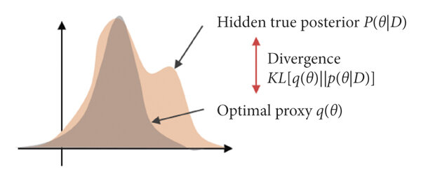
Reminder on the ELBO and KL divergence
We recall the decomposition of the marginal log-likelihood as a sum of the ELBO and the KL divergence for any distribution \(q\) over the latent variables:
\[\log p(\textbf{y} \mid \Theta ) = \mathcal{L}(q; \Theta) + KL \big( q \mid \mid p(\boldsymbol{\mu}, \boldsymbol{Z} \mid \textbf{y}, \Theta)\big)\]
The Evidence Lower Bound (ELBO) is a fundamental concept in variational inference, providing a lower bound on the log marginal likelihood of observed data. It is defined as:
\[\mathcal{L}(q; \Theta) = \mathbb{E}_{q} \big[ \log p(\textbf{y}, \boldsymbol{\mu} , \mathbf{Z}\mid \Theta) \big] - \mathbb{E}_{q} \big[ \log q( \boldsymbol{\mu} , \mathbf{Z}) \big]\]
where \(q( \boldsymbol{\mu} , \mathbf{Z})\) is an approximating distribution over the latent variables \( \boldsymbol{\mu} \) and \(\mathbf{Z}\).
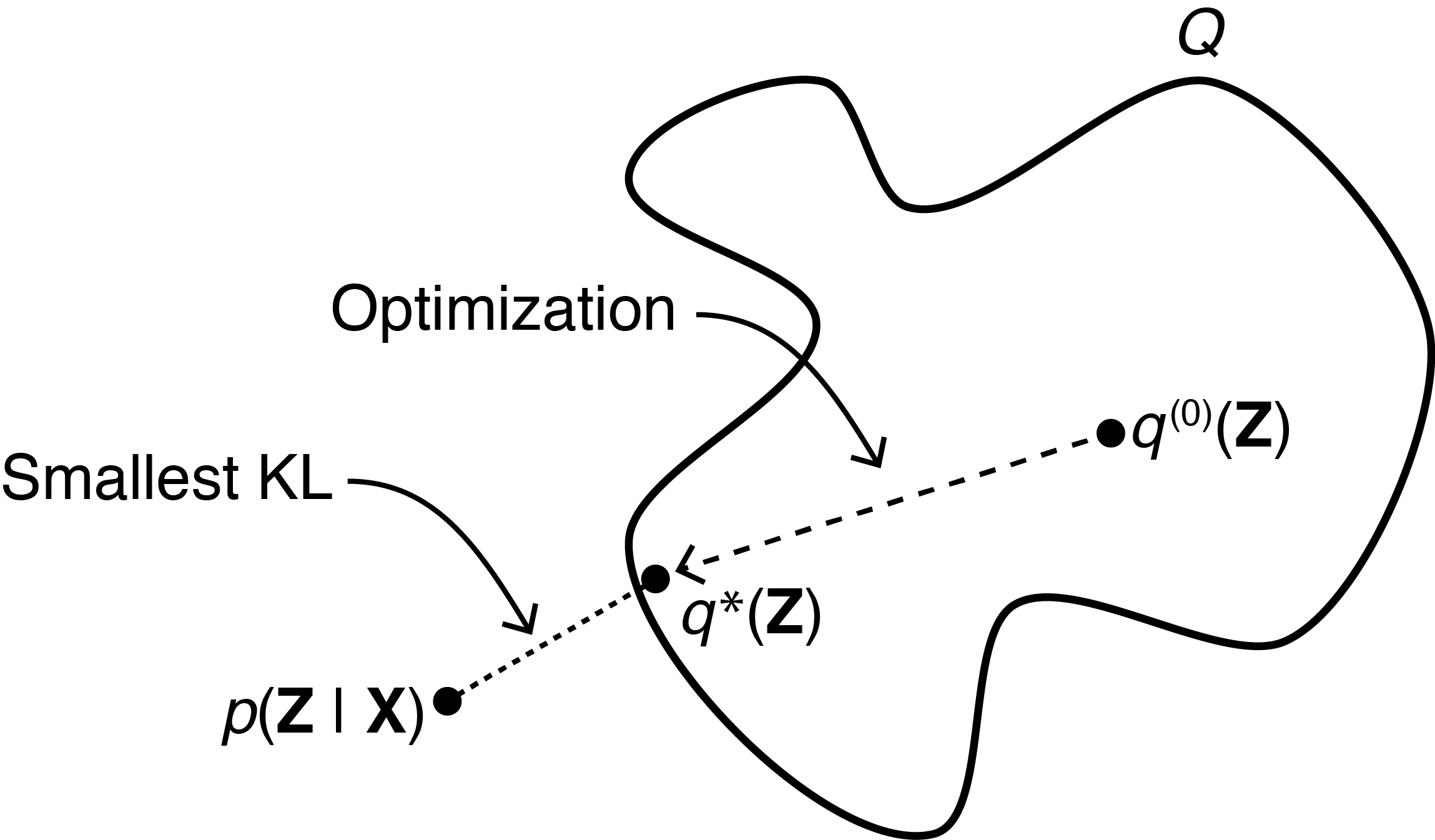
Variational inference : main idea
Contrarily to the EM algorithm, we cannot compute the true posterior \(p( \boldsymbol{\mu} , \mathbf{Z}\mid \textbf{y}, \Theta)\) in closed-form anymore, and set \(q( \boldsymbol{\mu} , \mathbf{Z})\) to this value so that the KL divergence vanishes.
![]()
We now need to optimise over a family of distributions \(\mathcal{Q}\) to find the best approximation \(\hat{q}( \boldsymbol{\mu} , \mathbf{Z})\) that maximises the ELBO.
Variational inference: mean-field approximation
A common choice is to consider a mean-field approximation, where the variational distribution factorises over groups of latent variables. In our case, we can assume independence between the cluster-specific mean processes \( \boldsymbol{\mu} \) and the cluster assignments \(\mathbf{Z}\):
\[q(\boldsymbol{\mu}, \boldsymbol{Z}) = q_{\boldsymbol{\mu}}(\boldsymbol{\mu})q_{\boldsymbol{Z}}(\boldsymbol{Z}).\]
Thanks to this assumption, both factors naturally factorise over clusters and tasks respectively:
- \(q_{\boldsymbol{\mu}}(\boldsymbol{\mu}) = \prod\limits_{k = 1}^K q_{\mu_k}(\mu_k),\)
- \(q_{\boldsymbol{Z}}(\boldsymbol{Z}) = \prod\limits_{t = 1}^T q_{Z_t}(Z_t).\)
From there, we can derive closed-form updates for each factor by sequentially optimising the ELBO with respect to one factor while keeping the other fixed.
Variational EM algorithm
The principles of the EM algorithm can be adapted to the variational inference context, leading to the Variational EM algorithm. At each iteration, we perform two main steps:
- Variational E-step: Update the variational distribution \(q(\cdot)\) to maximise the ELBO, given the current estimates of the model parameters \(\Theta\). This can be done using either mean-field or free-form approximations, and thus involve closed-form updates or optimisation techniques.
\[ \hat{q} = arg \max_{q \in \mathcal{Q}} \mathcal{L}(q; \Theta) \]
- M-step: Update the model parameters \(\Theta\) to maximise the ELBO, given the current variational distribution \(q(\cdot)\).
\[ \hat{\Theta} = arg \max_{\Theta} \mathcal{L}(q; \Theta) \]
Variational EM for the mixture of GPs
E step: \[
\begin{align}
\hat{q}_{\boldsymbol{\mu}}(\boldsymbol{\mu}) &= \color{green}{\prod\limits_{k = 1}^K} \mathcal{N}(\mu_\color{green}{k};\hat{m}_\color{green}{k}, \hat{\textbf{C}}_\color{green}{k}) , \hspace{2cm}
\hat{q}_{\boldsymbol{Z}}(\boldsymbol{Z}) = \prod\limits_{t = 1}^T \mathcal{M}(Z_t;1, \color{green}{\boldsymbol{\tau}_t})
\end{align}
\]
M step:
\[
\begin{align*}
\hat{\Theta}
&= \underset{\Theta}{\arg\max} \sum\limits_{k = 1}^{K}\sum\limits_{t = 1}^{T}\tau_{tk}\ \mathcal{N} \left( \mathbf{y}_t; \ \hat{m}_k, \boldsymbol{\Psi}_{\color{blue}{\theta_t}, \color{blue}{\sigma_t^2}} \right) - \dfrac{1}{2} \textrm{tr}\left( \mathbf{\hat{C}}_k\boldsymbol{\Psi}_{\color{blue}{\theta_t}, \color{blue}{\sigma_t^2}}^{-1}\right) \\
& \hspace{1cm} + \sum\limits_{k = 1}^{K}\sum\limits_{t = 1}^{T}\tau_{tk}\log \color{green}{\pi_{k}}
\end{align*}
\]
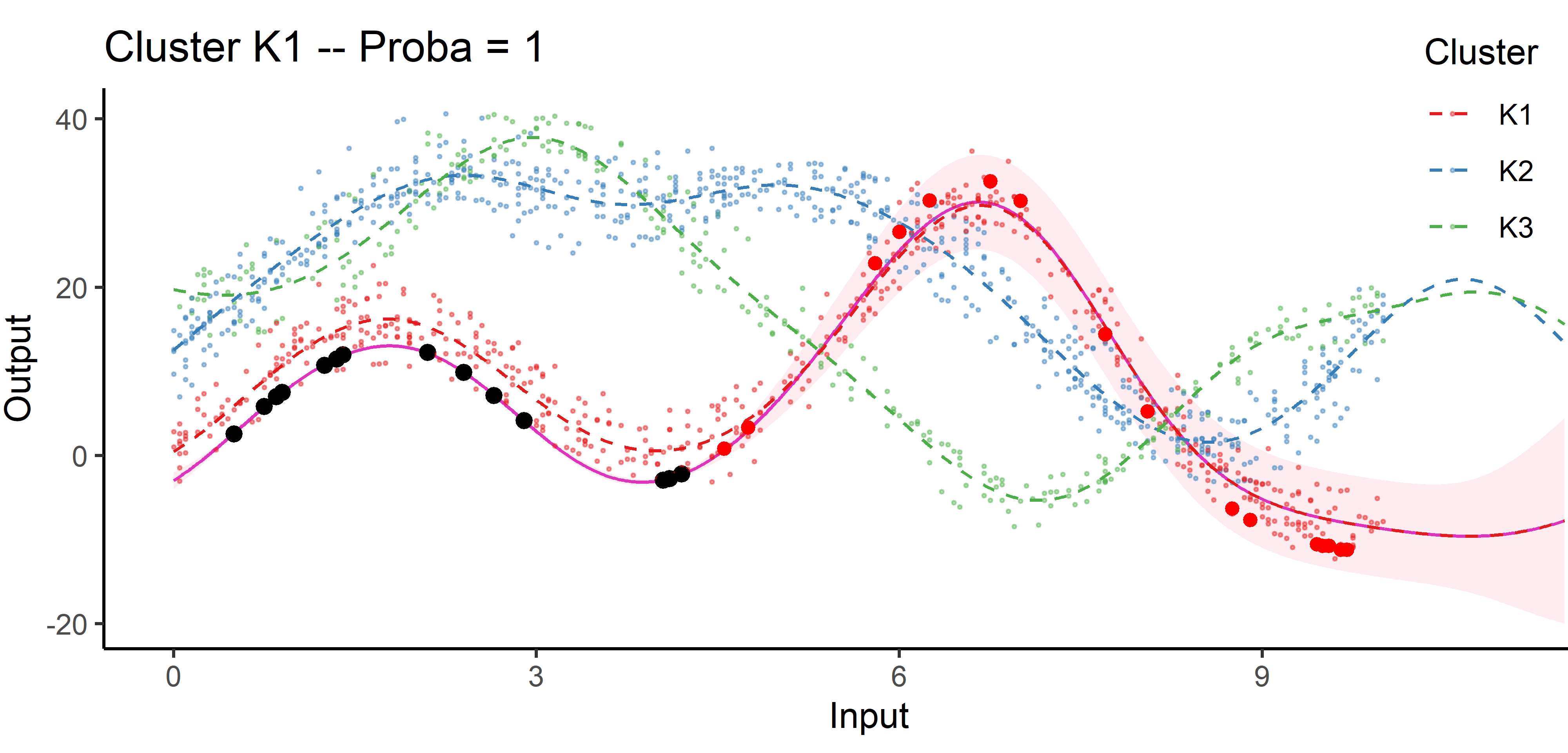
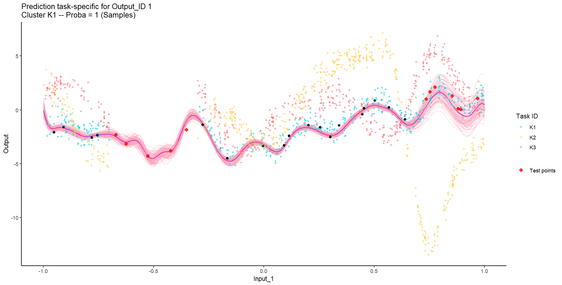
Cluster-specific and mixture predictions
- Multi-Task posterior for each cluster:
\[
p(y_*(\mathbf{x}^{p}) \mid \color{green}{Z_{*k}} = 1, y_*(\mathbf{x}_{*}), \textbf{y}) = \mathcal{N} \Big( y_*(\mathbf{x}^{p}); \ \hat{\mu}_{*}^\color{green}{k}(\mathbf{x}^{p}) , \hat{\Gamma}_{pp}^\color{green}{k} \Big), \forall \color{green}{k},
\]
\(\hat{\mu}_{*}^\color{green}{k}(\mathbf{x}^{p}) = \hat{m}_\color{green}{k}(\mathbf{x}^{p}) + \Gamma^\color{green}{k}_{p*} {\Gamma^\color{green}{k}_{**}}^{-1} (y_*(\mathbf{x}_{*}) - \hat{m}_\color{green}{k} (\mathbf{x}_{*}))\) \(\hat{\Gamma}_{pp}^\color{green}{k} = \Gamma_{pp}^\color{green}{k} - \Gamma_{p*}^\color{green}{k} {\Gamma^{\color{green}{k}}_{**}}^{-1} \Gamma^{\color{green}{k}}_{*p}\)
- Predictive multi-task GPs mixture:
\[p(y_*(\textbf{x}^p) \mid y_*(\textbf{x}_*), \textbf{y}) = \color{green}{\sum\limits_{k = 1}^{K} \tau_{*k}} \ \mathcal{N} \big( y_*(\mathbf{x}^{p}); \ \hat{\mu}_{*}^\color{green}{k}(\textbf{x}^p) , \hat{\Gamma}_{pp}^\color{green}{k}(\textbf{x}^p) \big).\]
An image is still worth many words
![]()
A unique mean process can struggle to capture relevant signals in presence of group structures.
An image is still worth many words
![]()
By identifying the underlying clustering structure, we can discard unnecessary information and provide enhanced predictions as well as lower uncertainty.
Saved by the weights
![]()
Each cluster-specific prediction is weighted by its membership probability \(\color{green}{\tau_{*k}}\).
Practical application: follow up of BMI during childhood
![]()
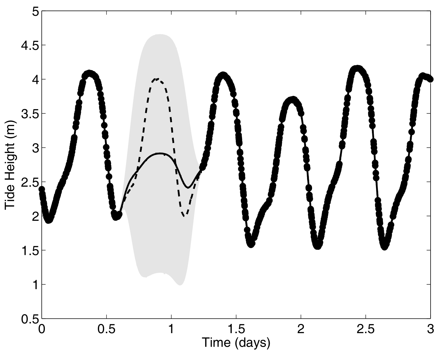
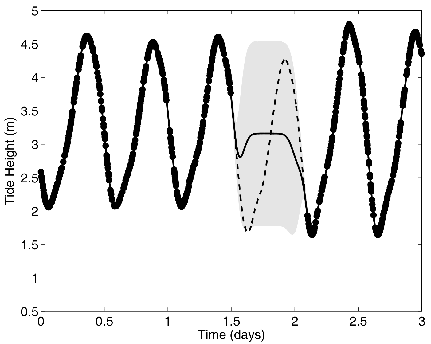
Reconstruction for sparse or incomplete data
![]()
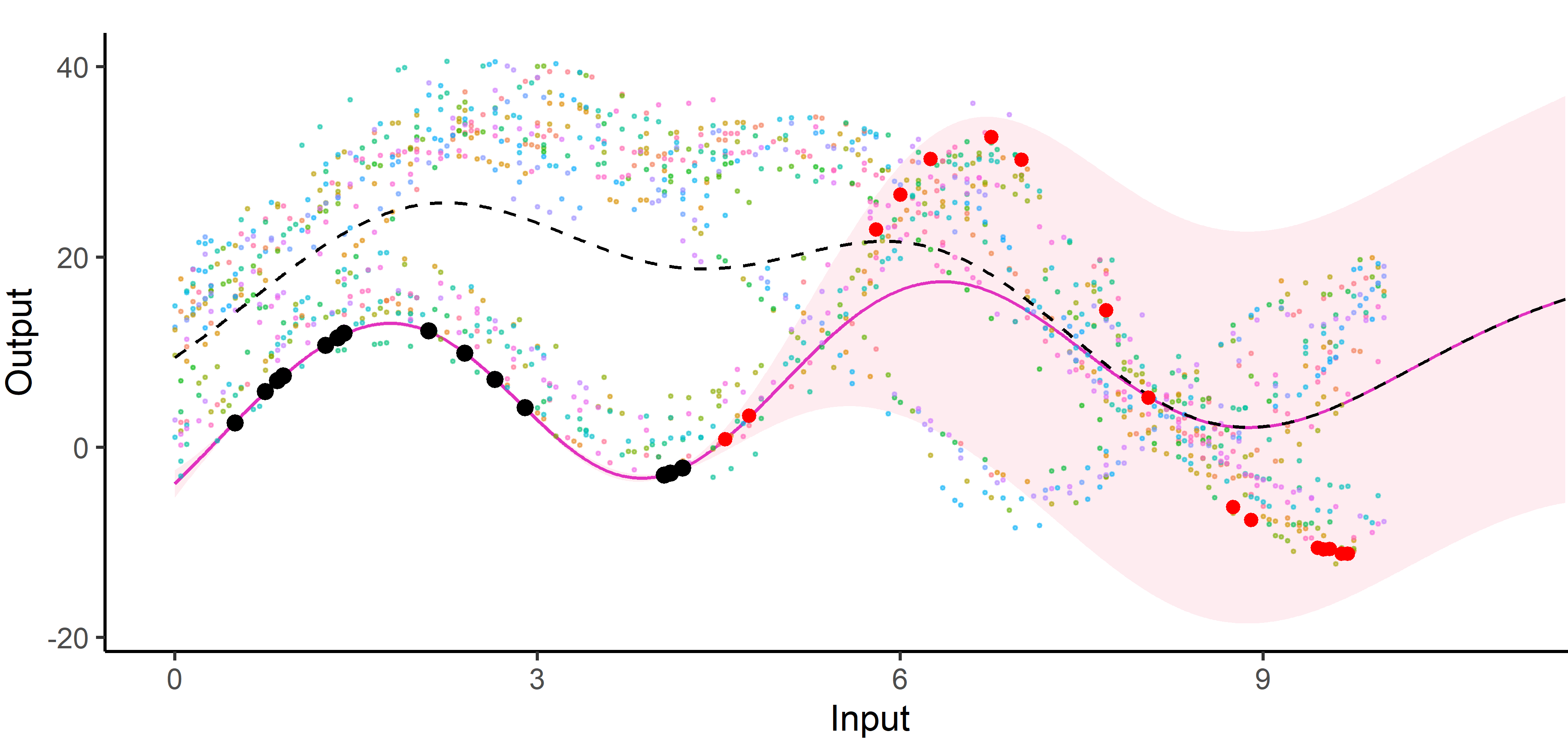
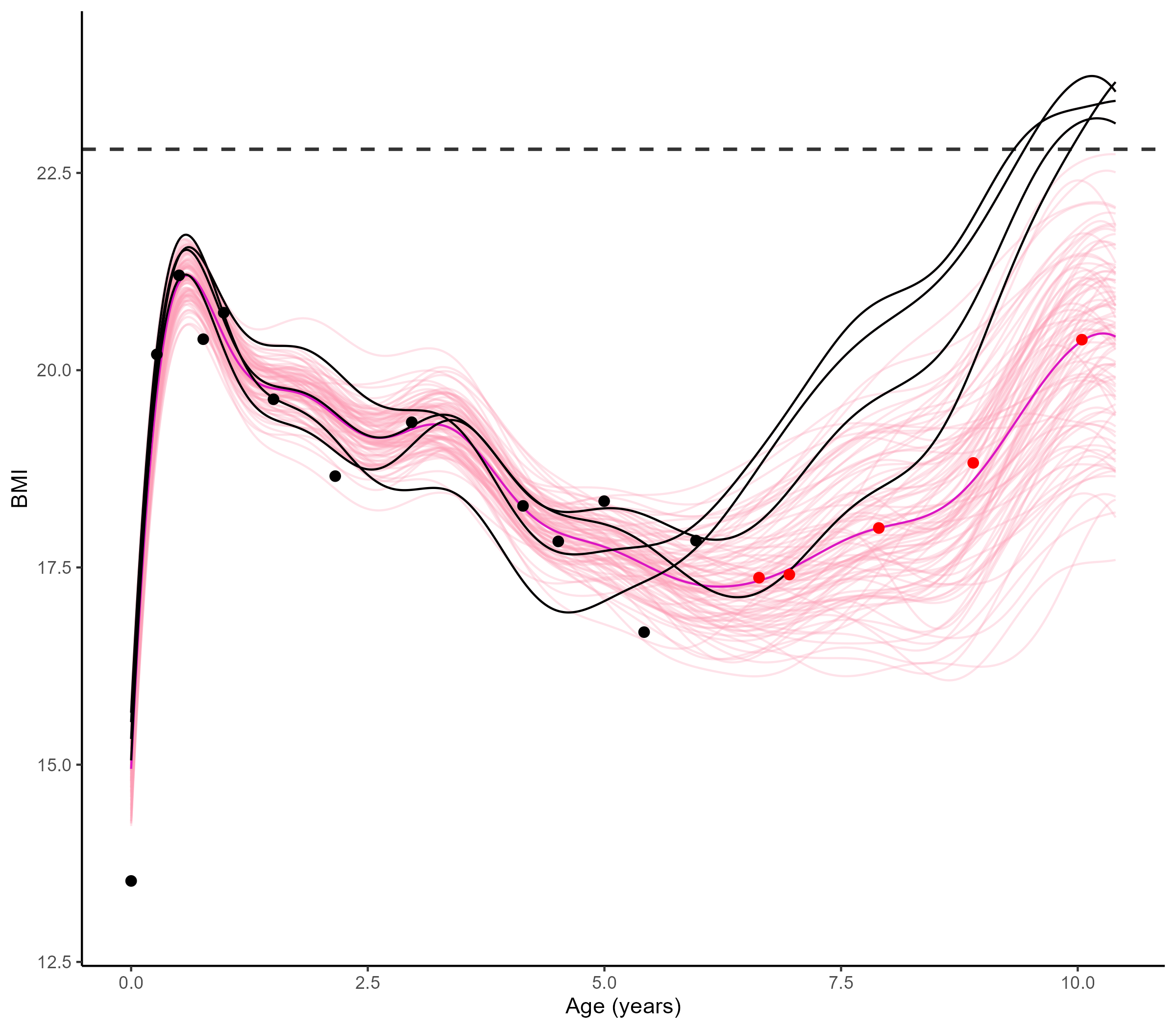
Forecasting long term evolution of BMI
![]()
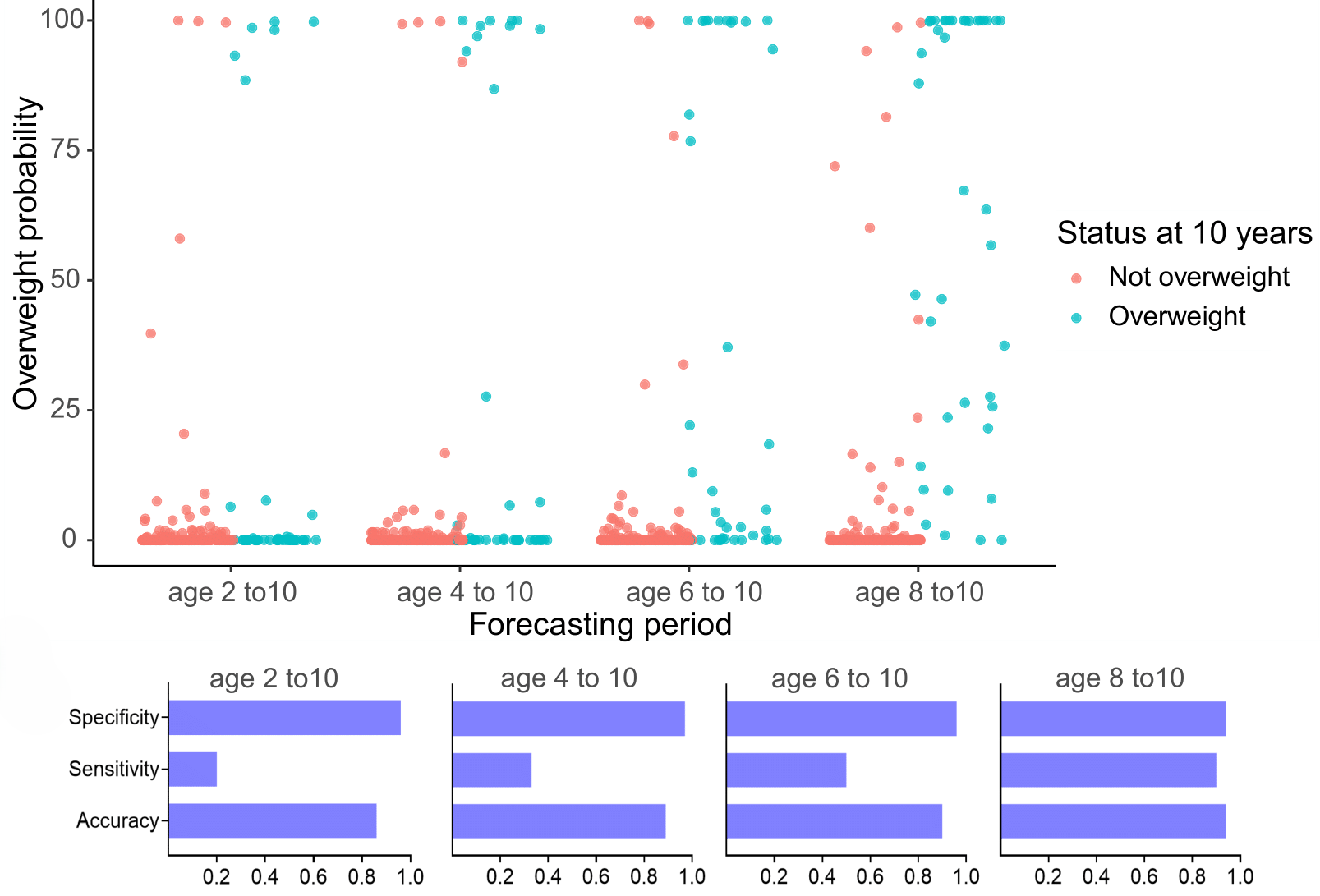
Leveraging the uncertainty quantification of GPs
![]()
Multi-Output GPs: another paradigm based on covariance structures
![]()
![]()
![]()
![]()
Multi-Task-Multi-Output GPs: best of both worlds?
- Multi-Output GPs derive full rank covariance matrices to exploit cross-correlations between all Input-Output pairs. They are flexible, expressive, and well-designed to recover very different signals or measurements. On the down side, they are computationally expensive, sometimes difficult to train in practice, and poorly adapted to modelling multiple tasks/individuals.
- Multi-Task GPs leverage latent mean processes to share information on the common trends and properties of the data. They are parsimonious, efficient, and well-designed to capture common patterns for multiple tasks/individuals on the same variable of interest. On the down side, they can be limited to fully capture correlations between the GPs and exploit initial knowledge that collected data may be of different natures.
Both work on separate parts of a GP, with no assumption on the other, and are theoretically compatible. They are even expected to synergise well, by tackling each others limitations.
Generative model of MOMT GPs
\[\begin{bmatrix} y_t^{1} \\ \vdots \\ y_t^{O} \\ \end{bmatrix} =
\begin{bmatrix} \mu_0 \\ \vdots \\ \mu_0 \\ \end{bmatrix} +
\begin{bmatrix} f_t^{1} \\ \vdots \\ f_t^{O} \\ \end{bmatrix} +
\begin{bmatrix} \epsilon_t^{1} \\ \vdots \\ \epsilon_t^{O} \\ \end{bmatrix}, \hspace{3cm} \forall t = 1, \dots, T\]
- \(\mu_0 \sim \mathcal{GP}(m_0, K_0),\)
- \(\begin{bmatrix} f_t^{1} \\ \vdots \\ f_t^{O} \\ \end{bmatrix} \sim \mathcal{GP}(0, \Sigma_{\theta_t}), \ \perp \!\!\! \perp_t,\)
- \(\begin{bmatrix} \epsilon_t^{1} \\ \vdots \\ \epsilon_t^{O} \\ \end{bmatrix} \sim \mathcal{GP}(0, \begin{bmatrix} {\sigma_t^{1}}^O \\ \vdots \\ {\sigma_{t}^O}^2 \\ \end{bmatrix} \times I_O), \ \perp \!\!\! \perp_t.\)
All mathematical objects from Multi-Task GPs are now extended with stacked Outputs.
Process convolution covariance structure and inference
\[\Big[k_{\theta_t}(\mathbf{x}, \mathbf{x}^{\prime})\Big]_{o,o'} = \dfrac{S_{t,o} \ S_{t,o{\prime}}}{(2\pi)^{D/2} \ |\Sigma|^{1/2}} \ \exp\Big(-\dfrac{1}{2}(\mathbf{x} - \mathbf{x}^{\prime})^T \Sigma^{-1}(\mathbf{x}-\mathbf{x}^{\prime})\Big)\]
with:
- \(S_{t,o}, S_{t,o{\prime}} \in \mathbb{R}\), the Output-specific variance terms,
- \(\Sigma = P_{t,o}^{-1}+P_{t,o^{\prime}}^{-1}+\Lambda^{-1} \in \mathbb{R}^{D \times D}\).
These matrices are typically diagonal, filled with Output-specific and latent lengthscales, one per Input dimension. In the end, we need to optimise \(\color{red}{O}\times \color{blue}{T} \times (3D+1)\) hyper-parameters.
E-step
\[
\begin{align}
p(\mu_0(\color{grey}{\mathbf{x}}) \mid \textbf{y}, \hat{\Theta})
= \mathcal{N}(\mu_0(\color{grey}{\mathbf{x}}); \hat{m}_0(\color{grey}{\textbf{x}}), \hat{\textbf{K}}^{\color{grey}{\textbf{x}}}),
\end{align}
\]
M-step
\[
\begin{align*}
\hat{\Theta}
&= \underset{\Theta}{\arg\max} \sum\limits_{t = 1}^{T}\left\{ \log \mathcal{N} \left( \mathbf{y}_t; \hat{m}_0(\color{purple}{\mathbf{x}_t^O}), \boldsymbol{\Psi}_{\theta_t, \sigma_t^2}^{\color{purple}{\mathbf{x}_t^O}} \right) - \dfrac{1}{2} Tr \left( \hat{\mathbf{K}}^{\color{purple}{\mathbf{x}_t^O}} {\boldsymbol{\Psi}_{\theta_t, \sigma_t^2}^{\color{purple}{\mathbf{x}_t^O}}}^{-1} \right) \right\}.
\end{align*}
\]
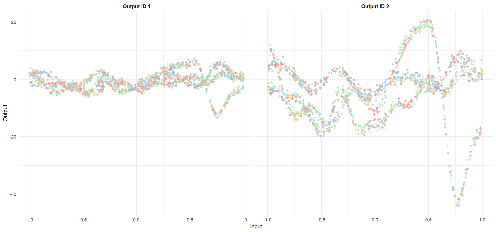
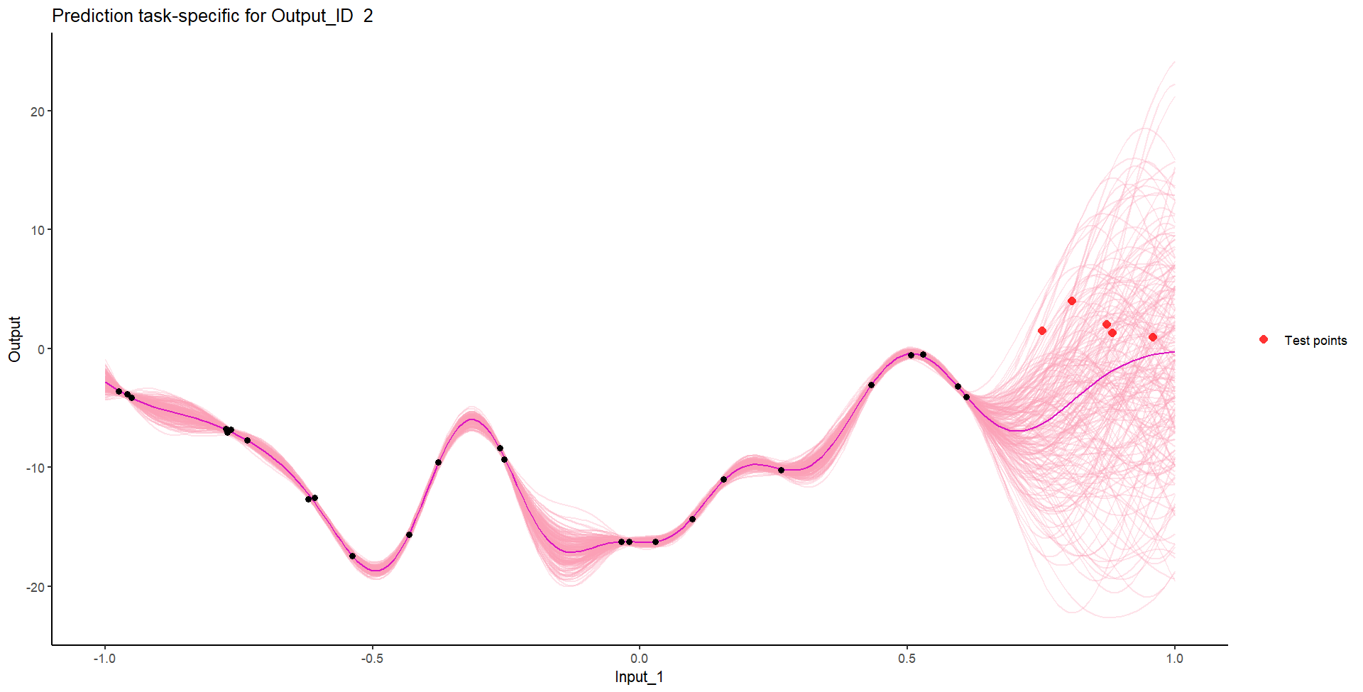
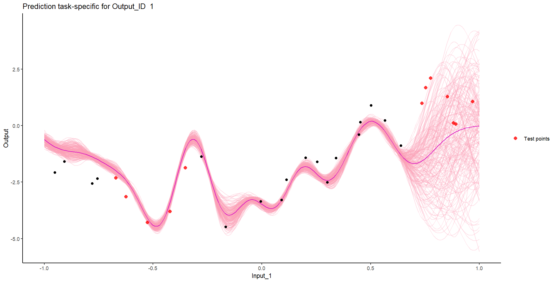
Let’s try something difficult
![]()
For instance, this context could correspond to measuring two distinct Outputs for several Tasks over time, gathered into unknown groups (that we want to recover), and for which we want to predict missing values of one Output, or forecast future values of both.
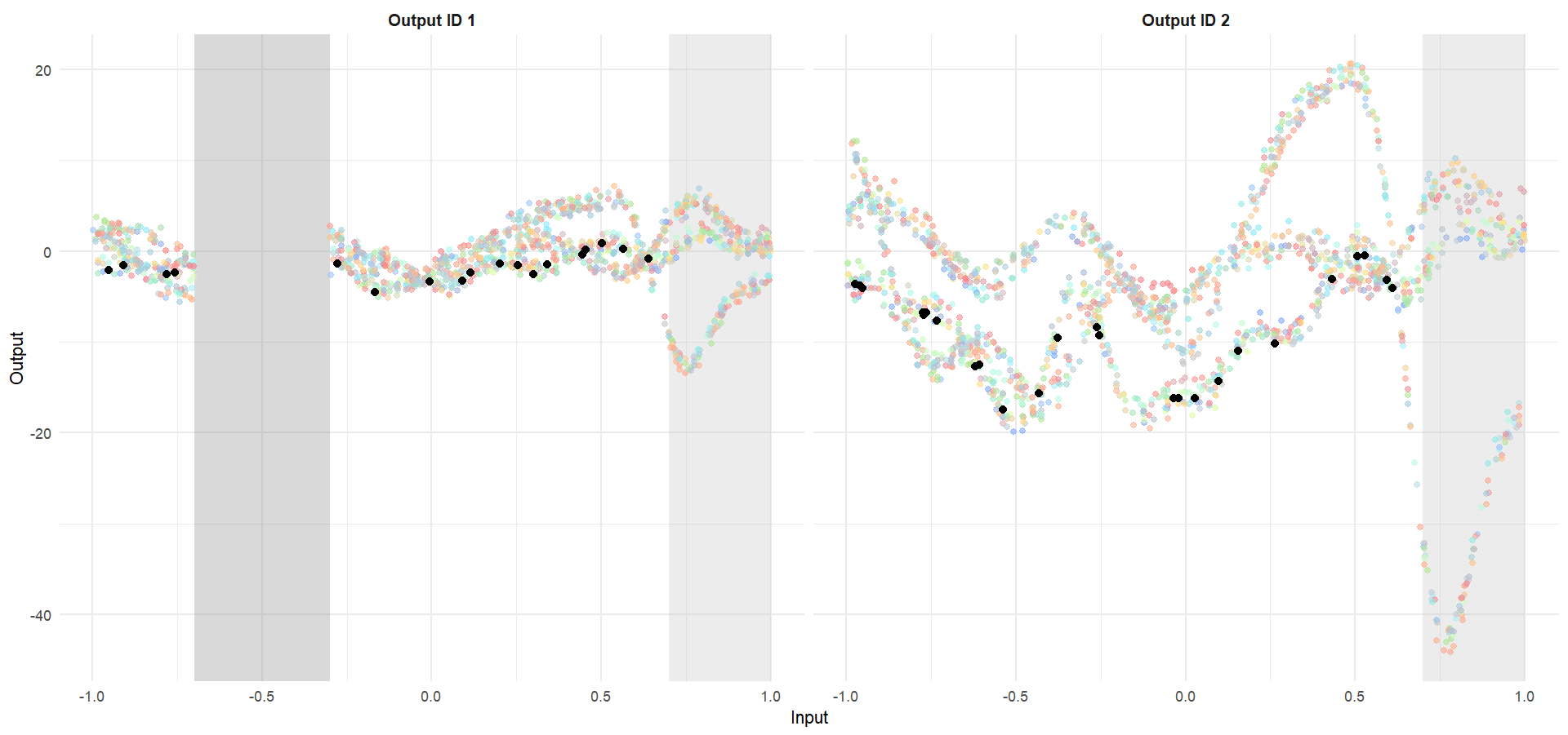
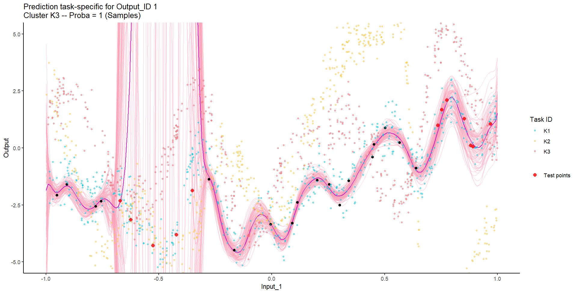
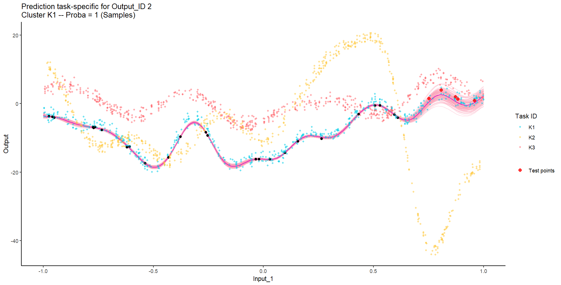
Let’s try something difficult
![]()
Let’s remove [-0.7, -0.3] of 2nd Output, and [0.7, 1] of both Outputs for the testing Task, and try to predict those testing points (and recover the underlying clusters).
We don’t even try vanilla GPs, maybe Multi-Output GPs?
Perhaps Multi-Task GPs can do better?
Do we really get the best of both worlds?
Take home messages
- Multi-Output / Multi-task: the same mathematical problem can hide different intuitions on the data and lead to dedicated modelling paradigms,
- Both the mean and covariance parameters can effectively be leveraged to share information,
- Modelling jointly data coming from several sources can costs roughly the same as independant modelling, but can improve dramatically predictive capacities.
Rule of thumb:
| Independant variables of interest |
Single-Task |
\(\color{red}{O}\times\mathcal{O}(N^3\) |
| Correlated variables of interest |
Multi-Output |
\(\mathcal{O}(\color{red}{O}^3 N^3)\) |
| Occurences of the same phenomenon |
Multi-Task |
\(\mathcal{O}(\color{blue}{T} \times N^3)\) |
| Occurences of correlated variables |
Multi-Task-Multi-Output |
\(\mathcal{O}(\color{blue}{T}\times\color{red}{O}^3 N^3)\) |

 https://distill.pub/2019/visual-exploration-gaussian-processes/