logo_inrae < logo_gpss >

Multi-Output and Multi-Task
Gaussian Processes

Arthur Leroy - GABI & MIA Paris Saclay, INRAE

Gaussian Process Summer School - 15/09/2026

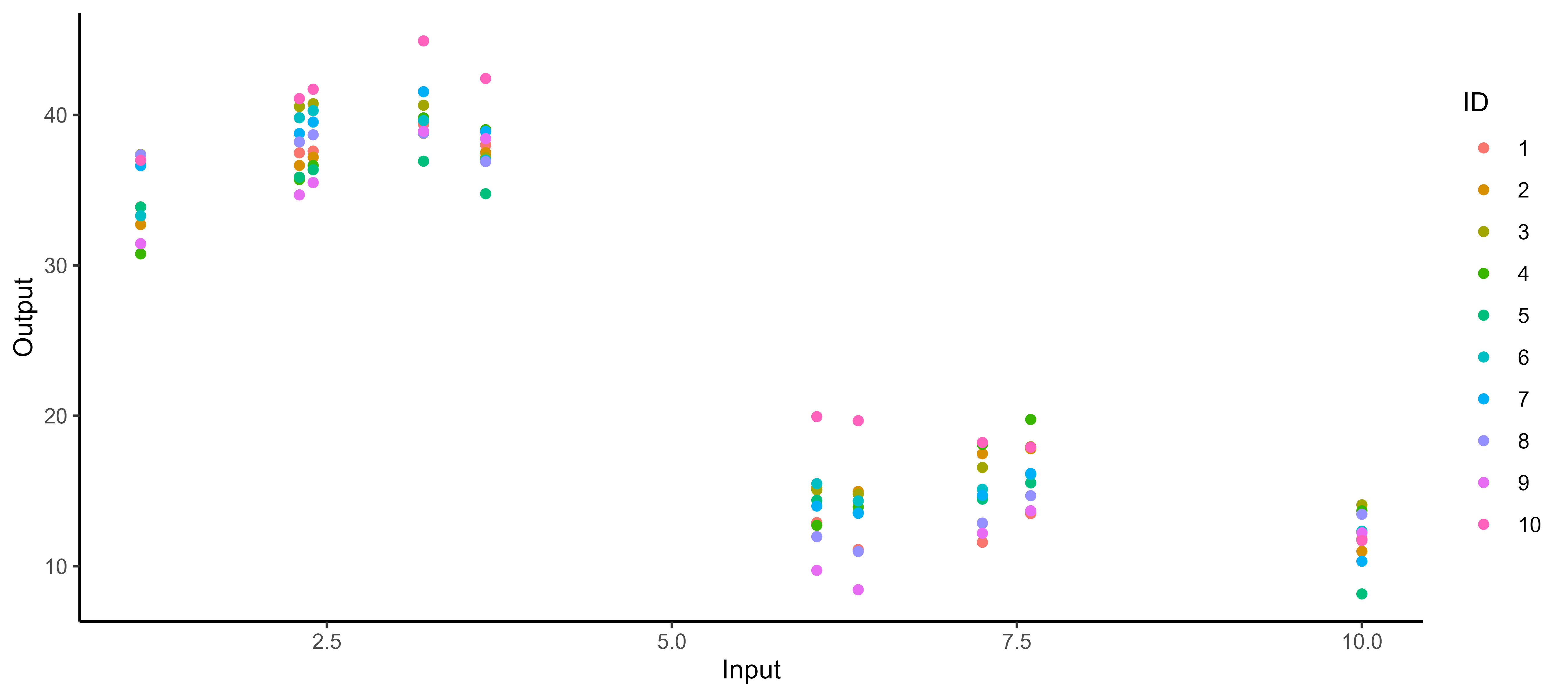
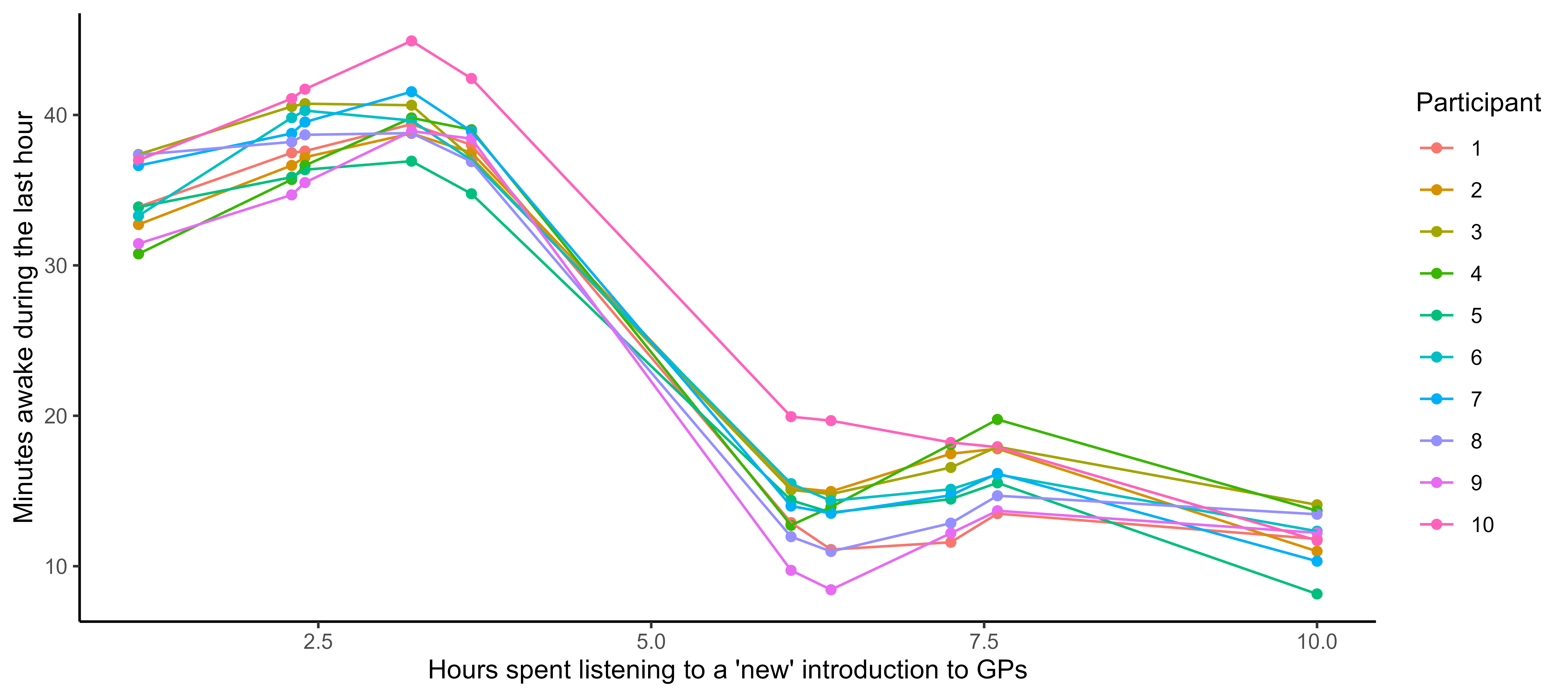
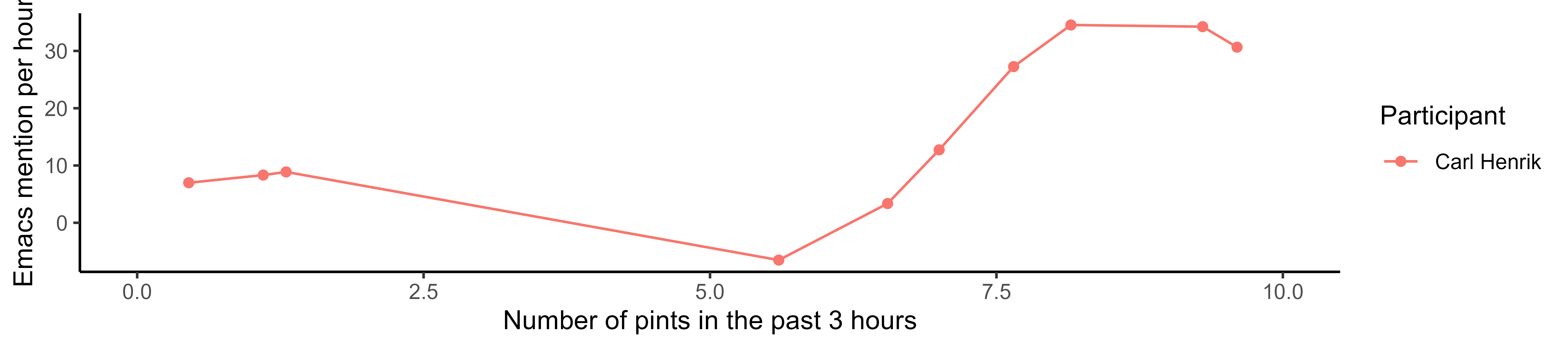
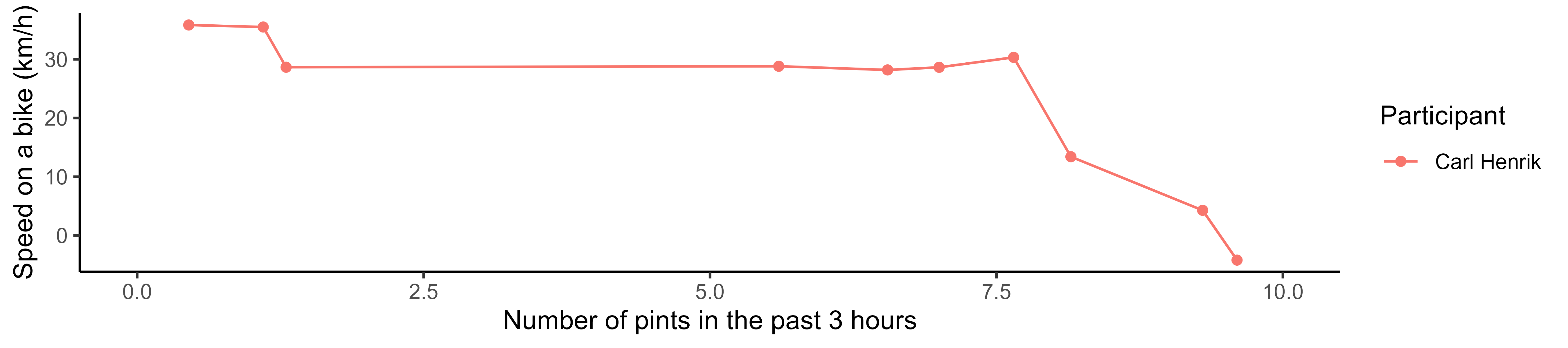
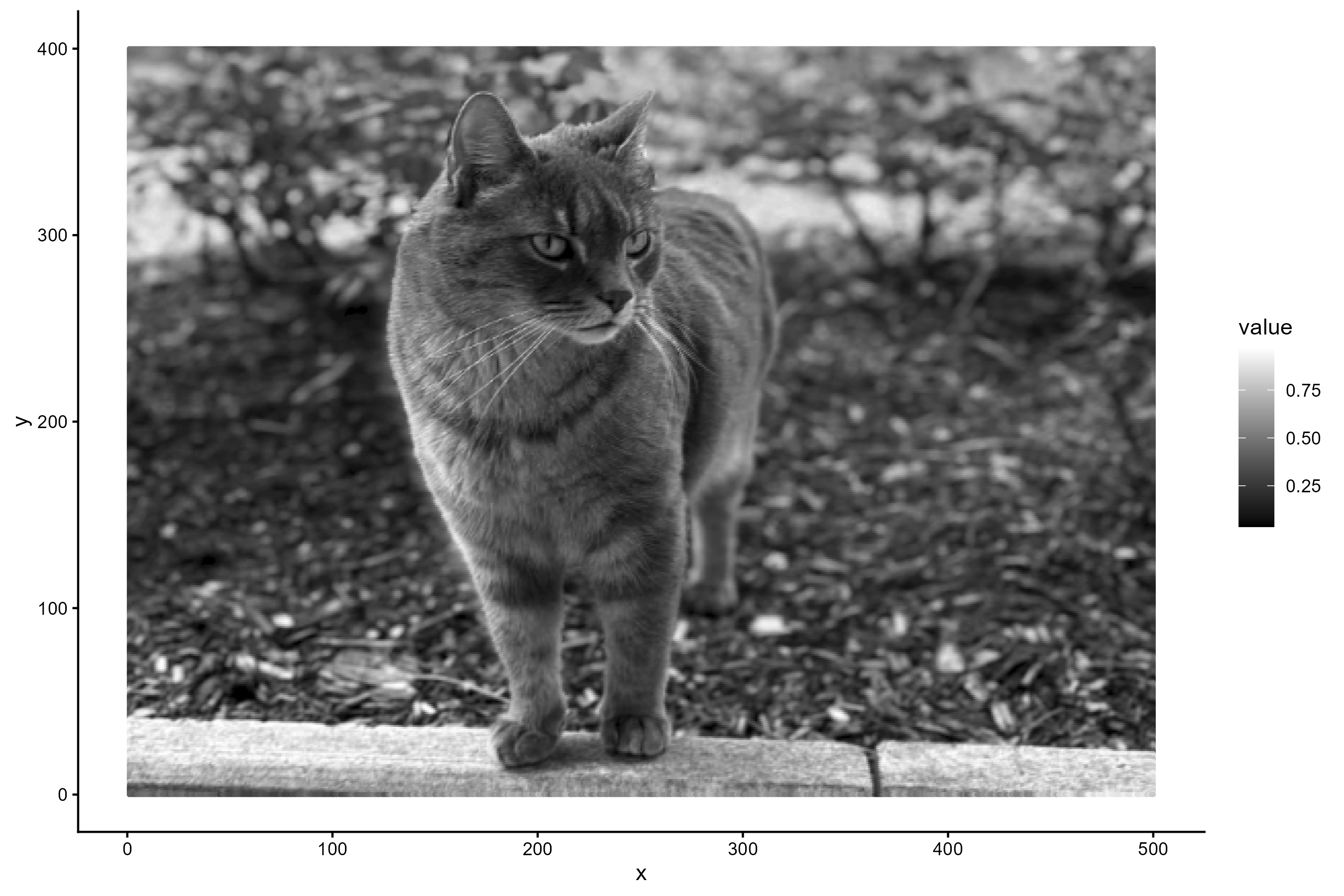
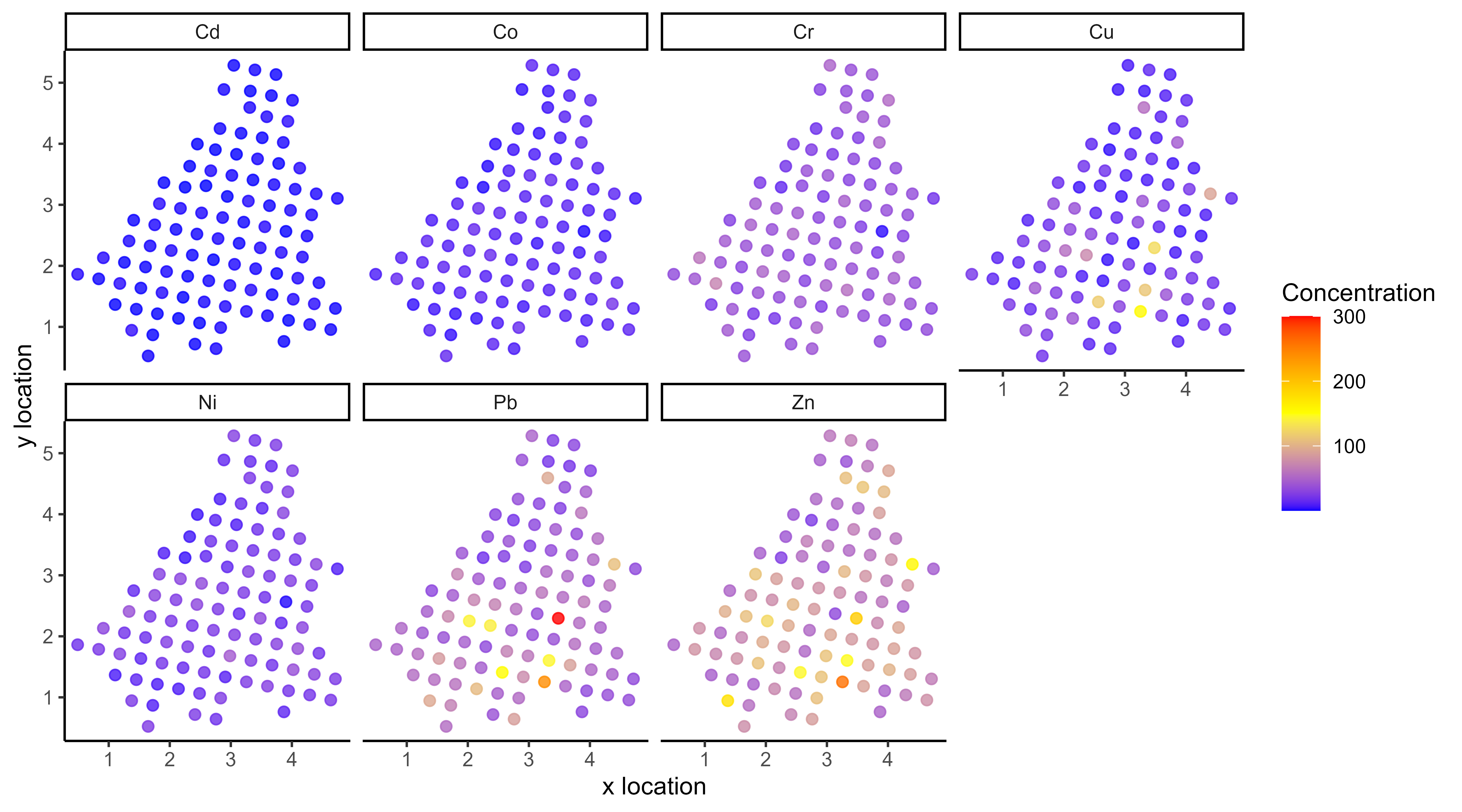
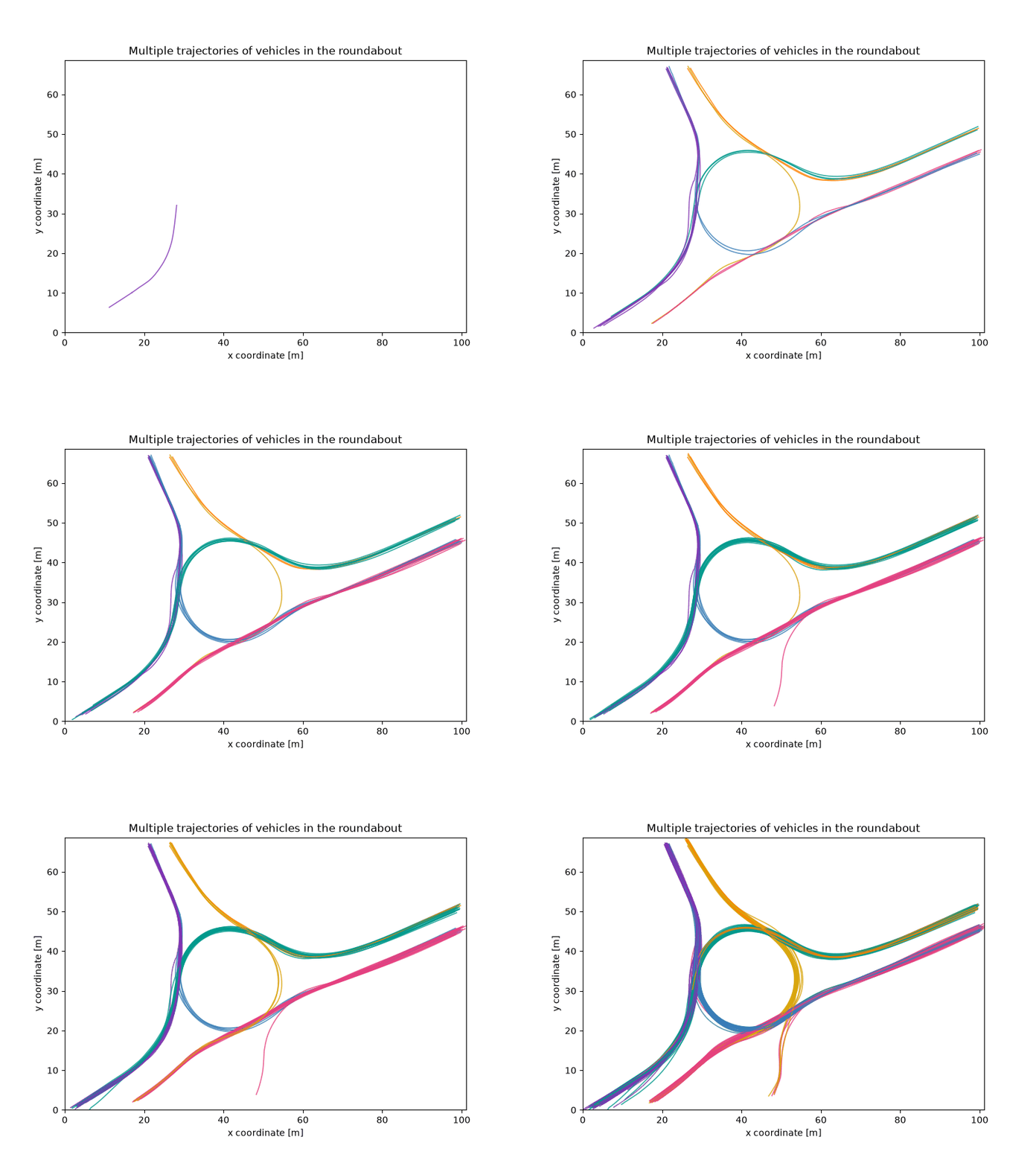
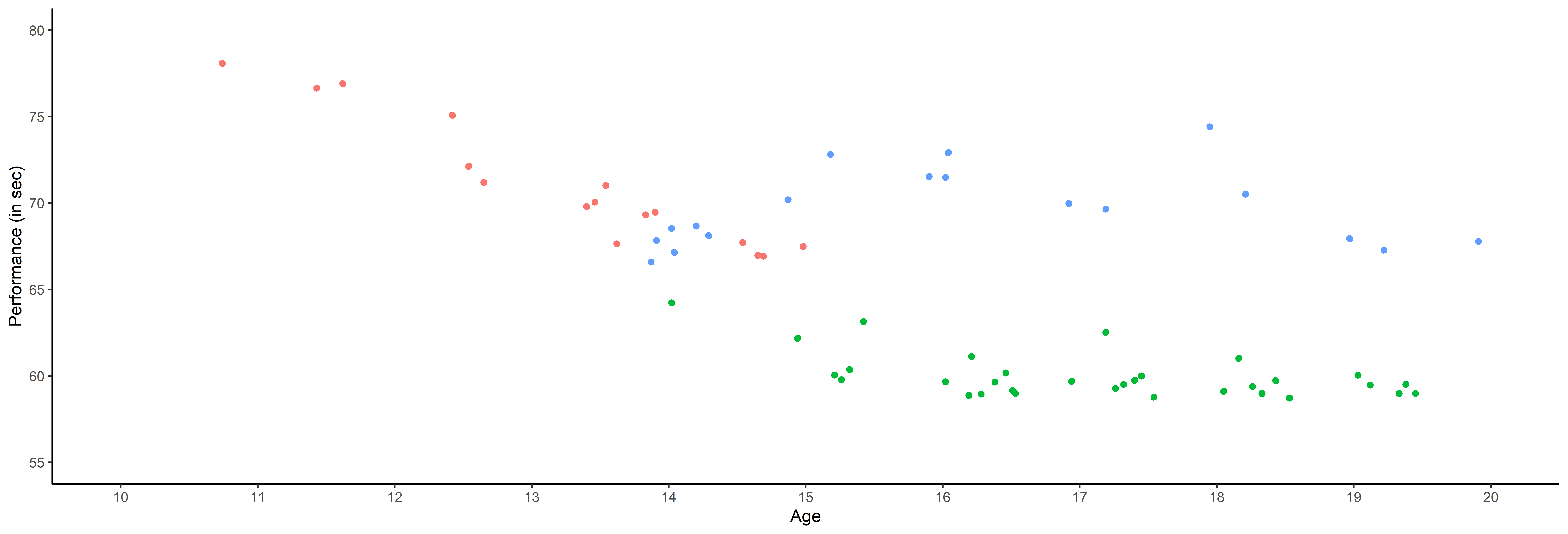
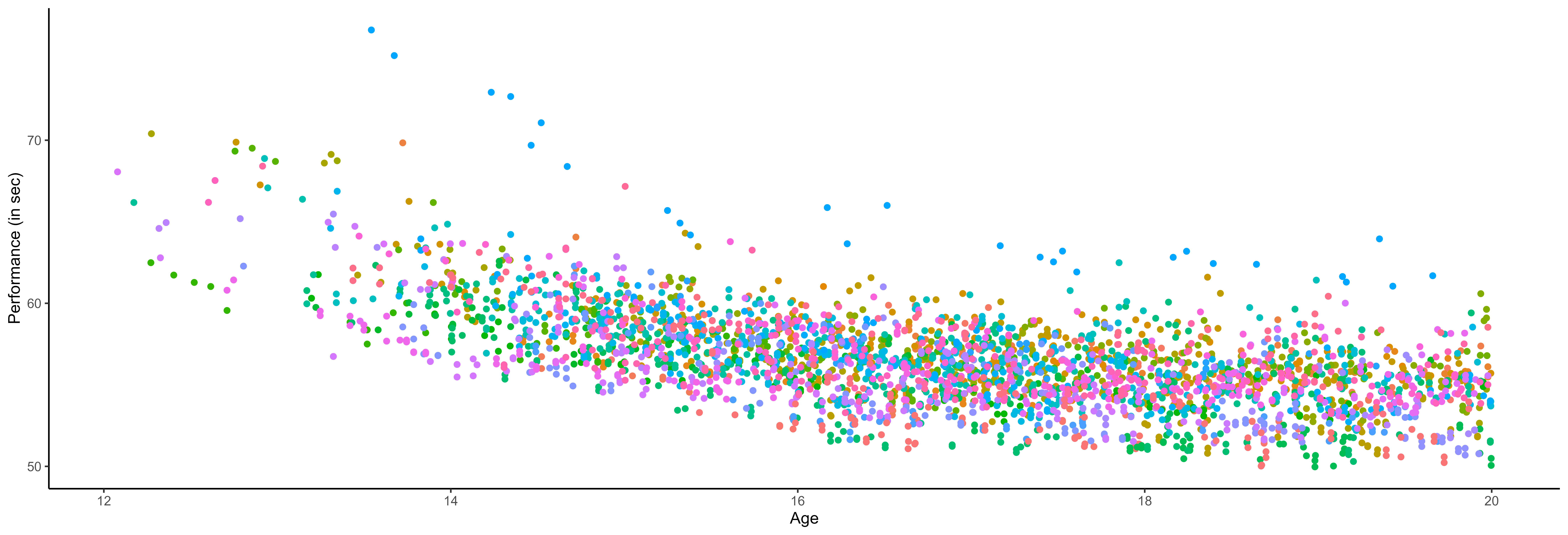
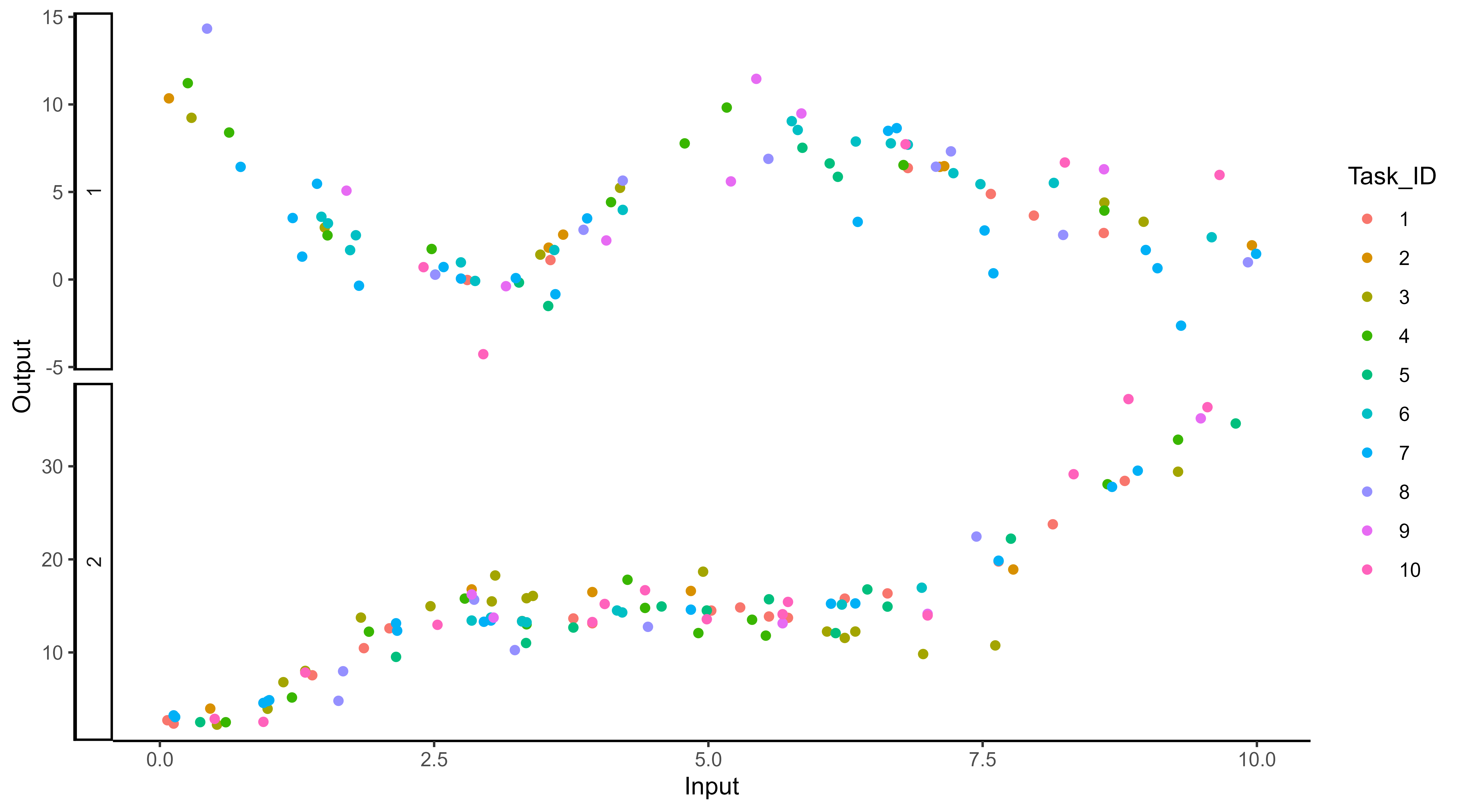
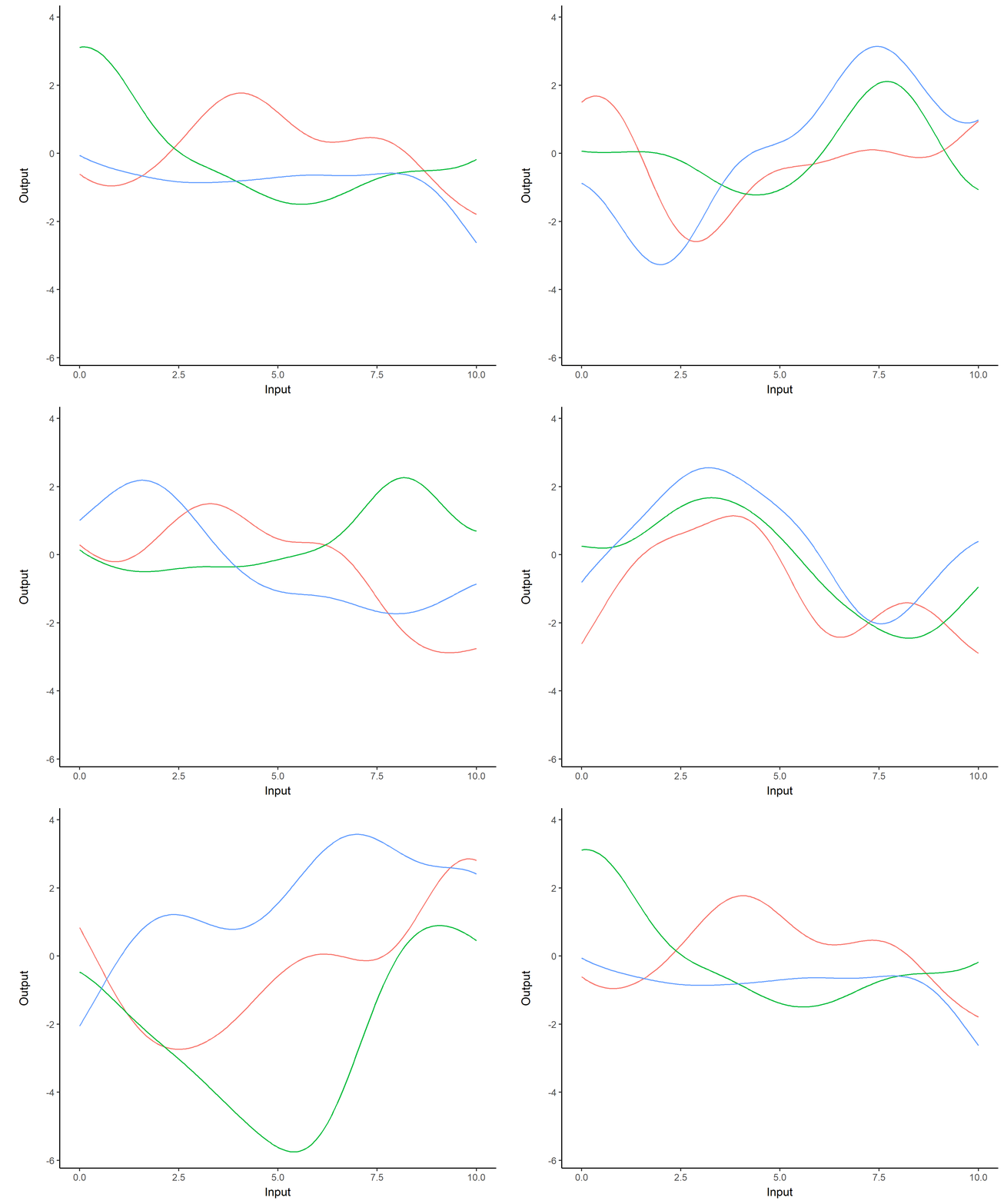
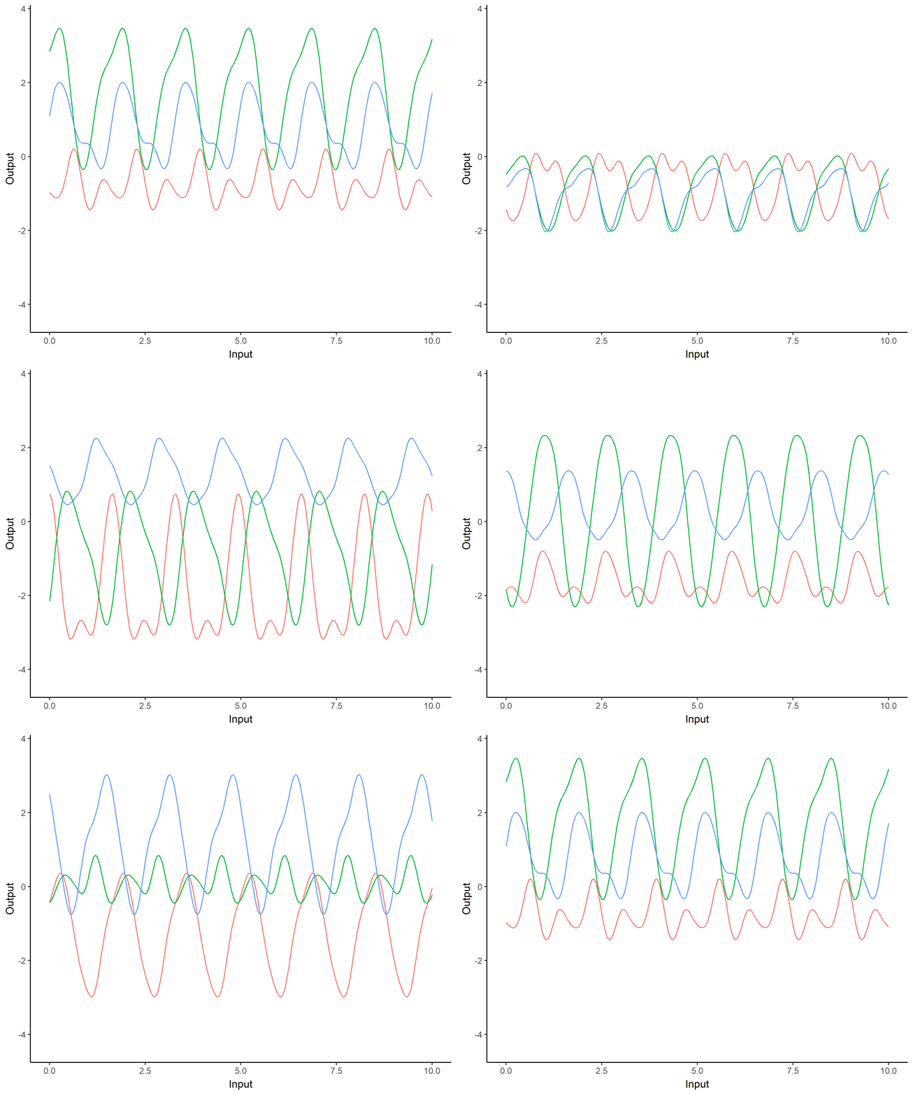
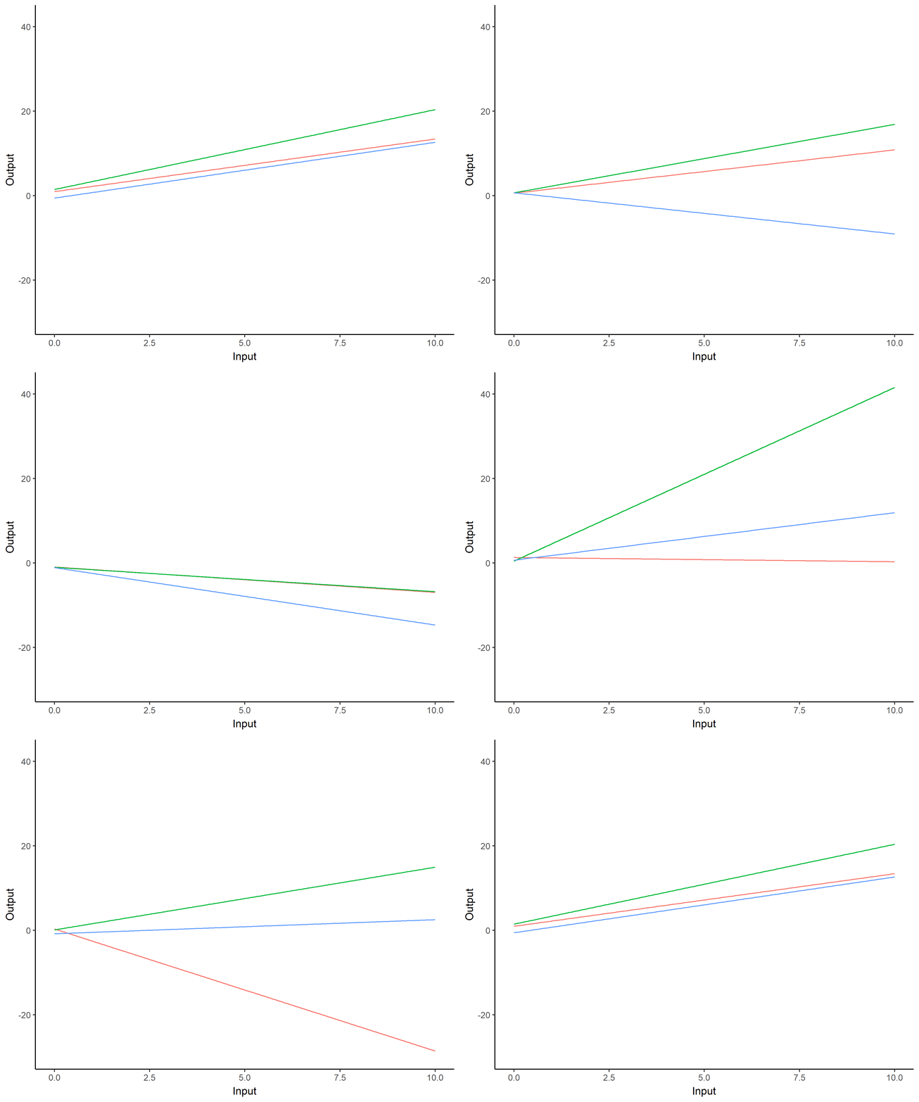
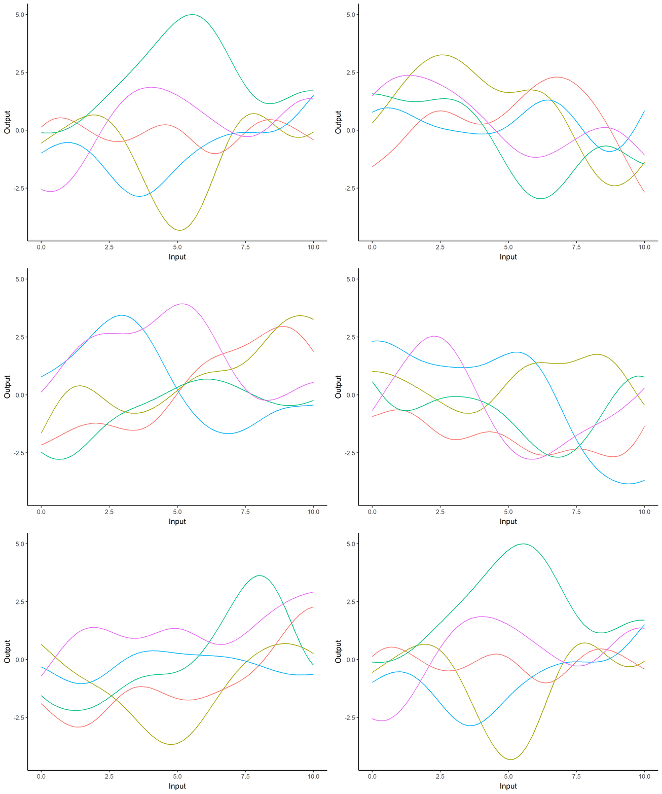
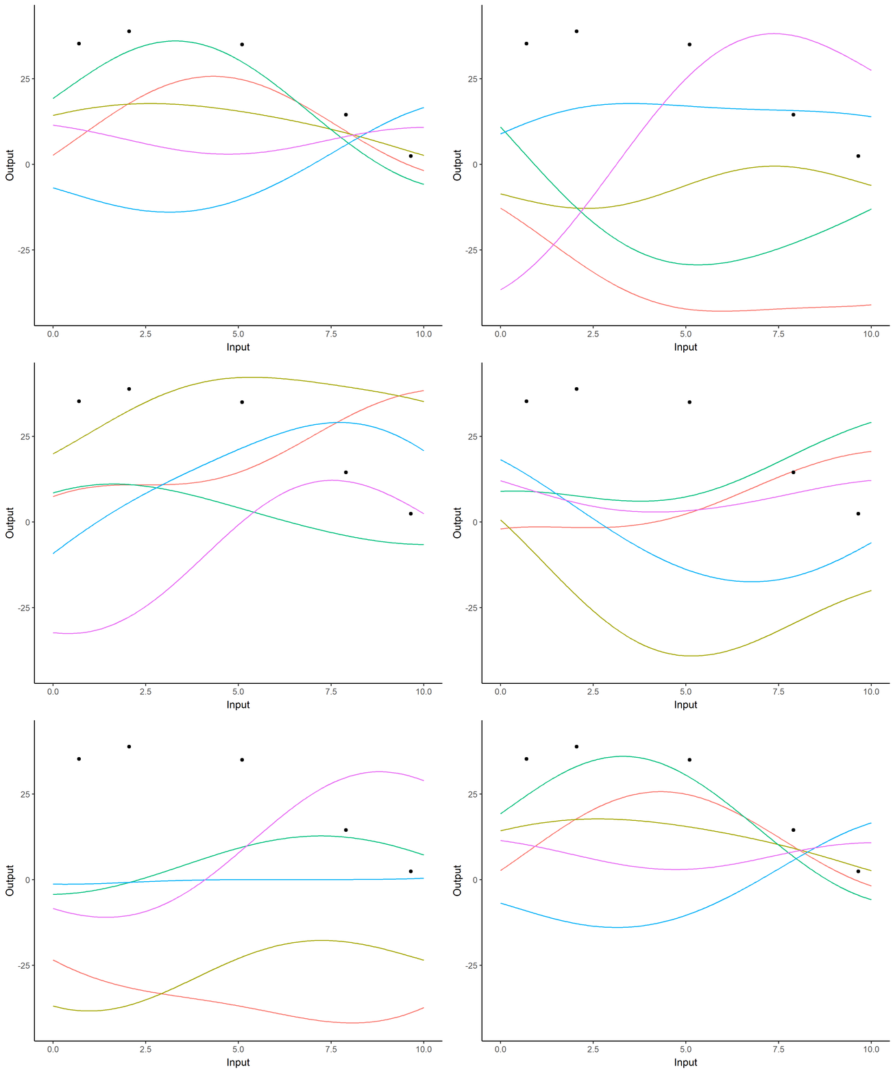
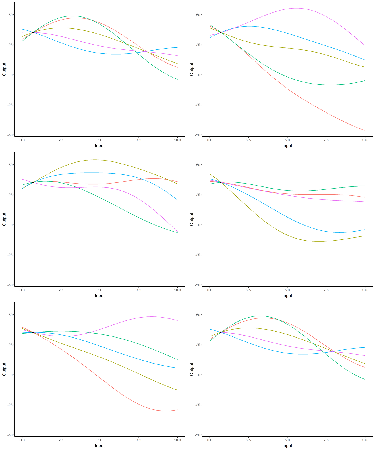
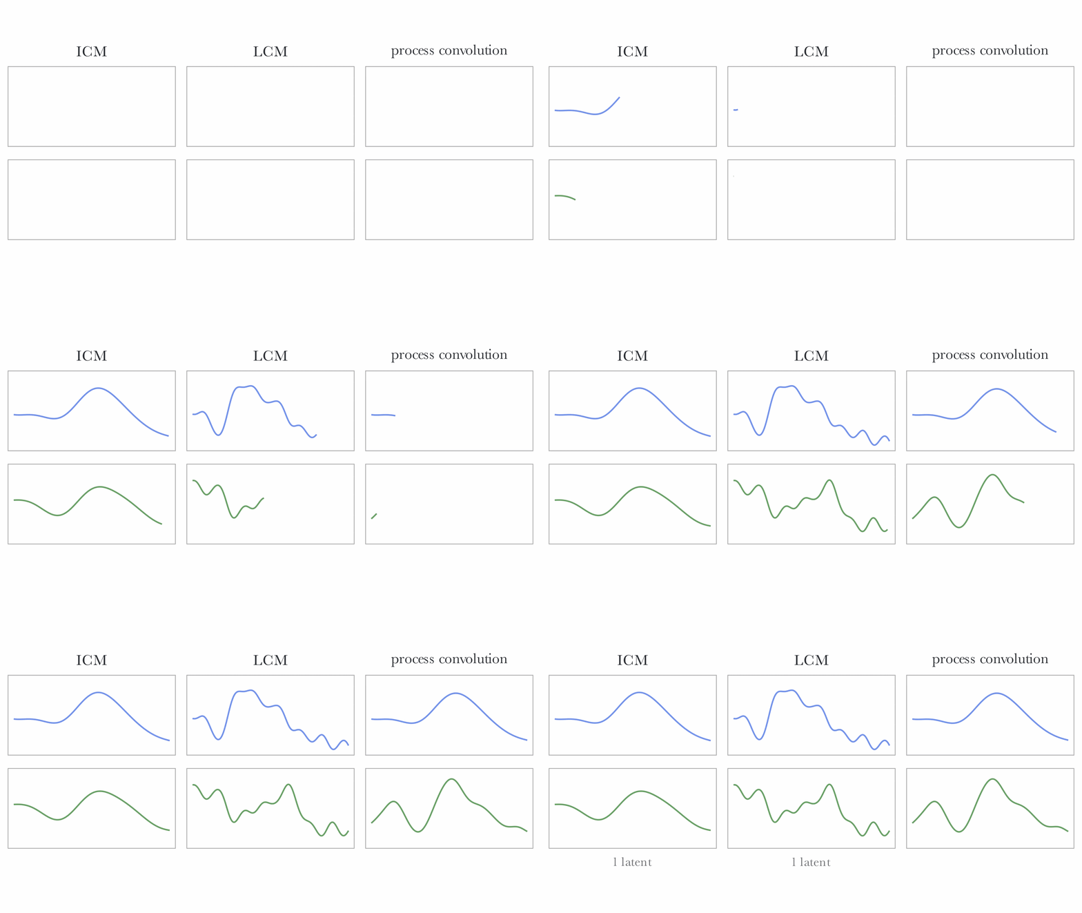
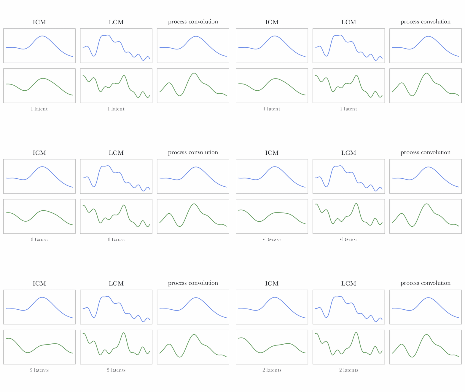
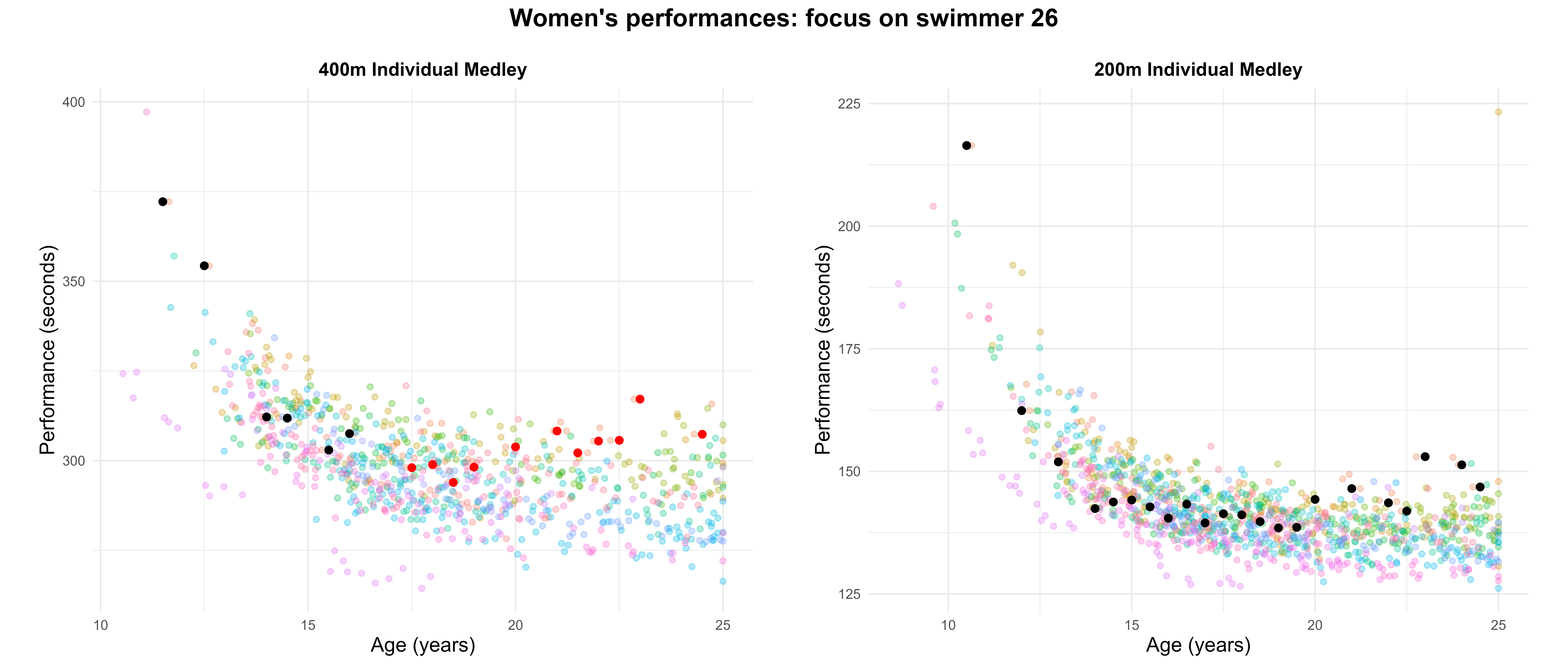
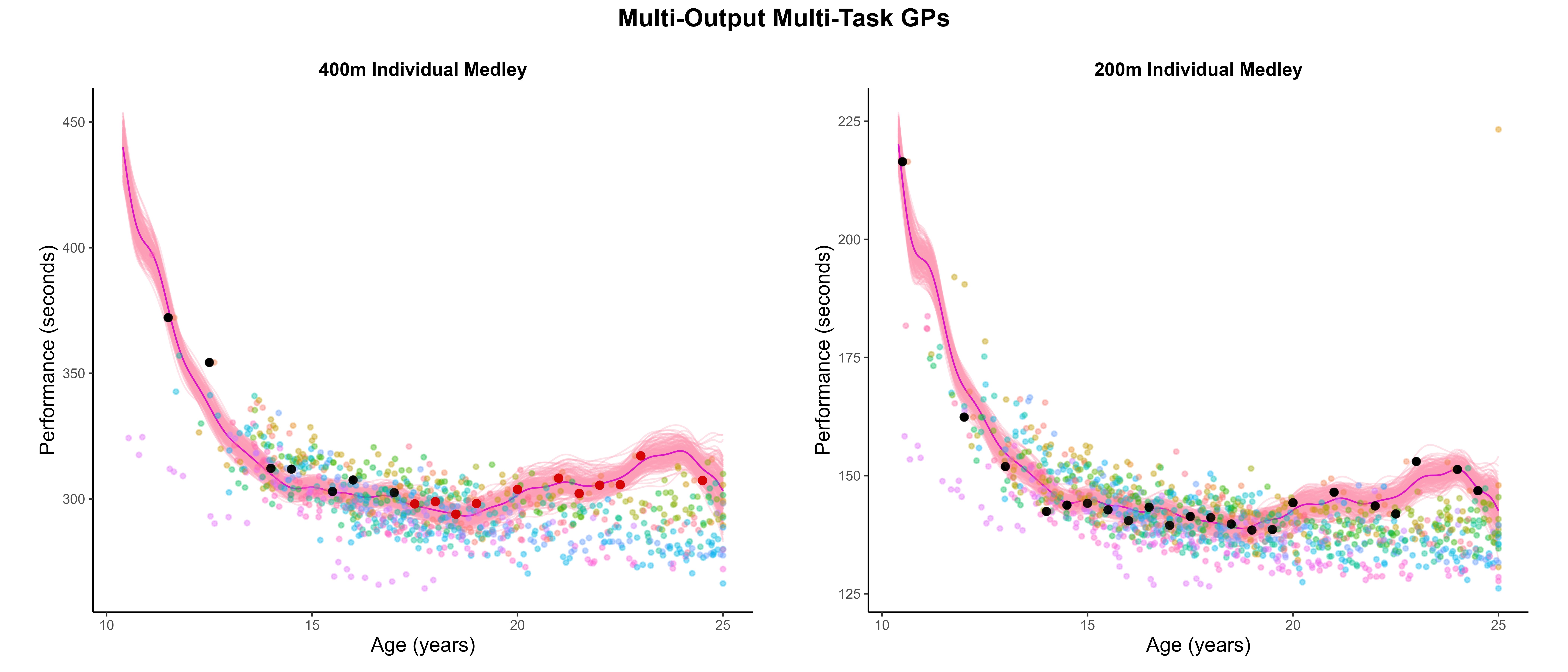
It all starts with observations from multiple sources …

… but sometimes we are not measuring the same things …

Let’s play a game

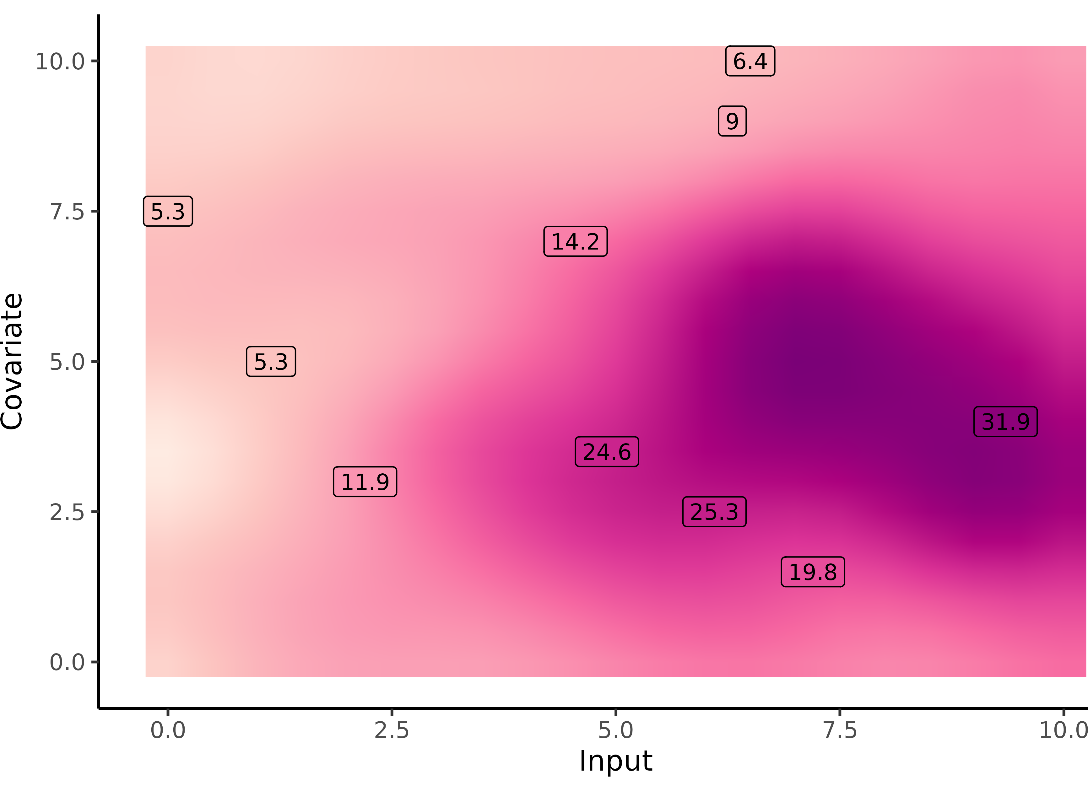
A secret ambition of this talk is to clarify the differences between Inputs, Outputs, Tasks, Channels, and all the things in ML that, at first, are basically just columns of a dataset.

Name	Time	Location_x	Location_y	Heart_rate	Current_speed
Alice	09:00	12.4	8.1	72	1.2
Bob	09:00	5.2	14.7	81	1.5
Charlie	09:00	18.1	3.5	68	0.9
Alice	09:05	13.1	8.8	75	1.4
Bob	09:05	6.0	15.4	85	1.6
Charlie	09:05	18.5	4.0	70	1.1
Alice	09:10	14.0	9.6	79	1.6
Bob	09:10	6.9	16.2	88	1.8
Charlie	09:10	19.0	4.7	73	1.3
Alice	09:15	15.0	10.5	82	1.8

Can you propose sensible choices for this table, and the subsequent data sets? Let’s argue folks!

So. We restart with observations from multiple sources …

… but sometimes we are not measuring the same things …

… sometimes data come in successive batches …

But it’s worth gathering them all!

… many things can be multidimensional …

… I feel like we are spiraling …

… among many other difficulties …

Irregular time series (in number of observations and location),
A few observations for each source,

… among many other difficulties …

Irregular input measurements (in number of observations and location),
A few observations for each source,
Many different sources.

… or all of them at once.

Multi-Task? Multi-Output? A proposed formalisation

In the previous examples, we saw a variety of situations that naturally lead to the same mathematical formulation of the learning problem:

\[y_s = \color{orange}{f_s}(x_s) + \epsilon_s, \hspace{3cm} \forall s = 1, \dots, S\]

Learn \(\color{orange}{f_s}\), the underlying relationship between \(x_s\) and \(y_s\), for each source of data \(\color{orange}{s}\).

Multi-, in contrast with single-, regression implies that some information can be shared across data sources to improve learning/predictions.

The nature of measurements leads to a more philosophical distinction:

Multi-Output should refer to several variables of interest. An Output is a quantity we aim to infer/predict from Input measurements, and which may be correlated with others.
Multi-Task implies the existence of an underlying pattern, shared by several tasks or individuals, which can be jointly exploited to build a common model.

Gaussian process: a prior distribution over functions

\[y = \color{orange}{f}(x) + \epsilon\]

No restrictions on \(\color{orange}{f}\) but a prior distribution on a functional space: \(\color{orange}{f} \sim \mathcal{GP}(m(\cdot),C(\cdot,\cdot))\)

While \(m\) is often assumed to be \(0\), the covariance structure is critical and defined through tailored kernels.

Gaussian process: all you need is a posterior

The Gaussian property induces that unobserved points have no influence on inference:

\[ \int \underbrace{p(f_{\color{grey}{obs}}, f_{\color{purple}{mis}})}_{\mathcal{GP}(m, C)} \ \mathrm{d}f_{\color{purple}{mis}} = \underbrace{p(f_{\color{grey}{obs}})}_{\mathcal{N}(m_{\color{grey}{obs}}, C_{\color{grey}{obs}})} \]

This crucial trick allows us to learn function properties from finite sets of observations. More generally, Gaussian processes are closed under conditioning and marginalisation.

\[\begin{bmatrix} f_{\color{grey}{o}} \\ f_{\color{purple}{m}} \\ \end{bmatrix} \sim \mathcal{N} \left( \begin{bmatrix} m_{\color{grey}{o}} \\ m_{\color{purple}{m}} \\ \end{bmatrix}, \begin{pmatrix} C_{\color{grey}{o, o}} & C_{\color{grey}{o}, \color{purple}{m}} \\ C_{\color{purple}{m}, \color{grey}{o}} & C_{\color{purple}{m, m}} \end{pmatrix} \right)\]

While marginalisation serves for training, conditioning leads the key GP prediction formula:

\[f_{\color{purple}{m}} \mid f_{\color{grey}{o}} \sim \mathcal{N} \Big( m_{\color{purple}{m}} + C_{\color{purple}{m}, \color{grey}{o}} C_{\color{grey}{o, o}}^{-1} (f_{\color{grey}{o}} - m_{\color{grey}{o}}), \ \ C_{\color{purple}{m, m}} - C_{\color{purple}{m}, \color{grey}{o}} C_{\color{grey}{o, o}}^{-1} C_{\color{grey}{o}, \color{purple}{m}} \Big)\]

Have you had enough introductions to GPs?

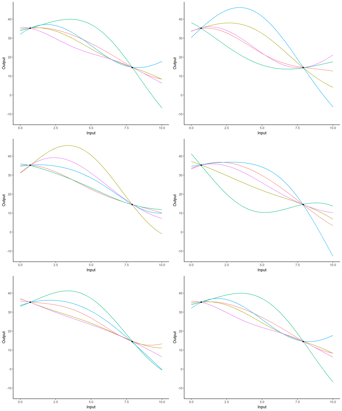
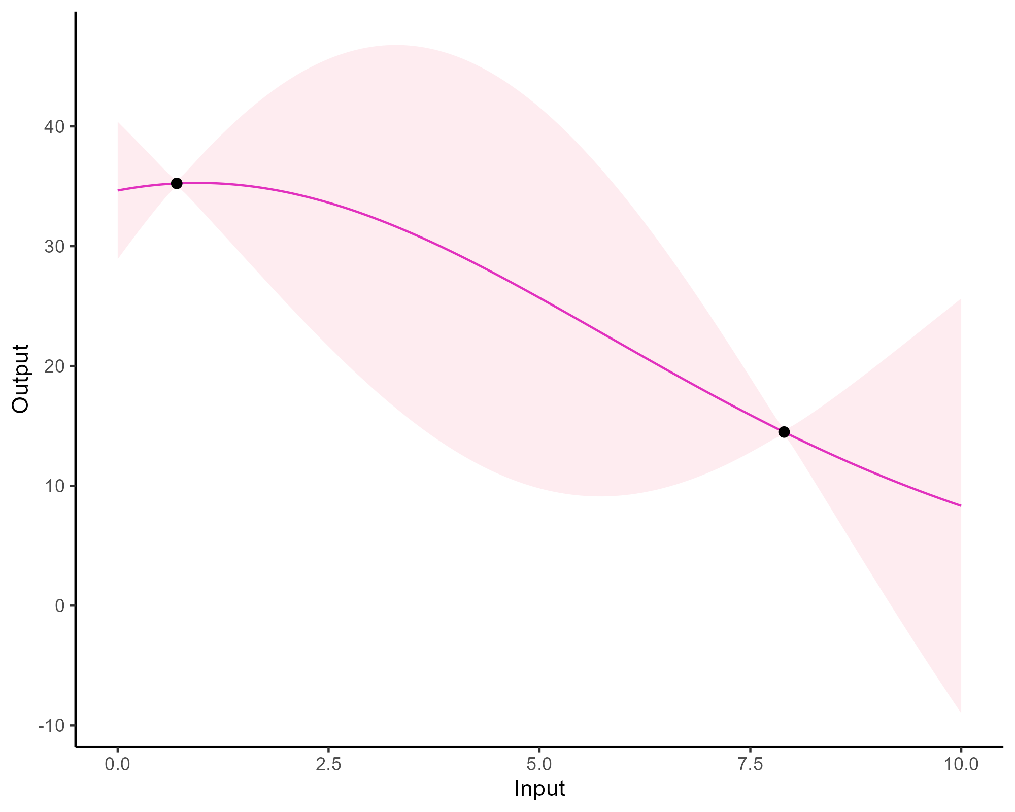
Another one for the road

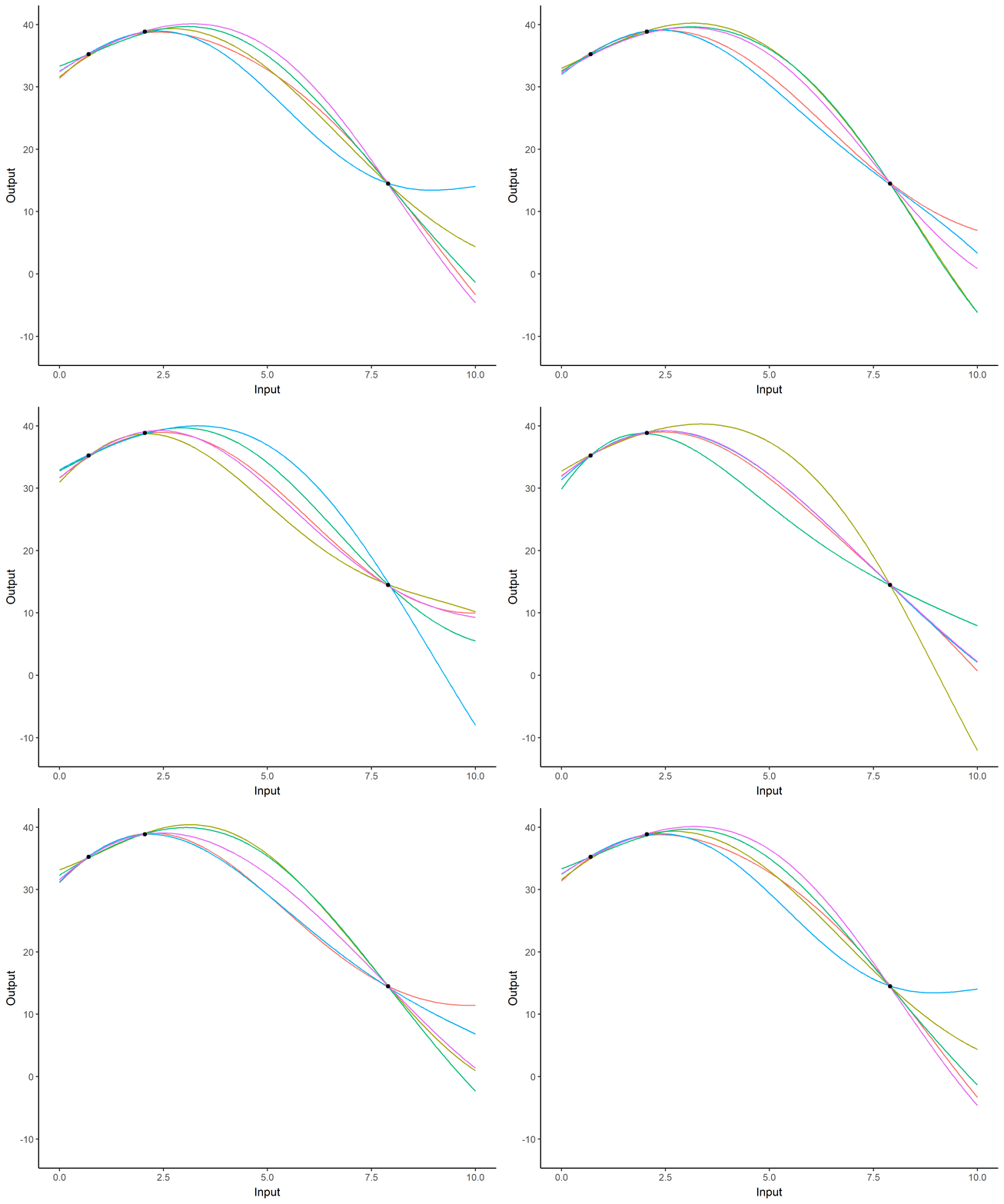
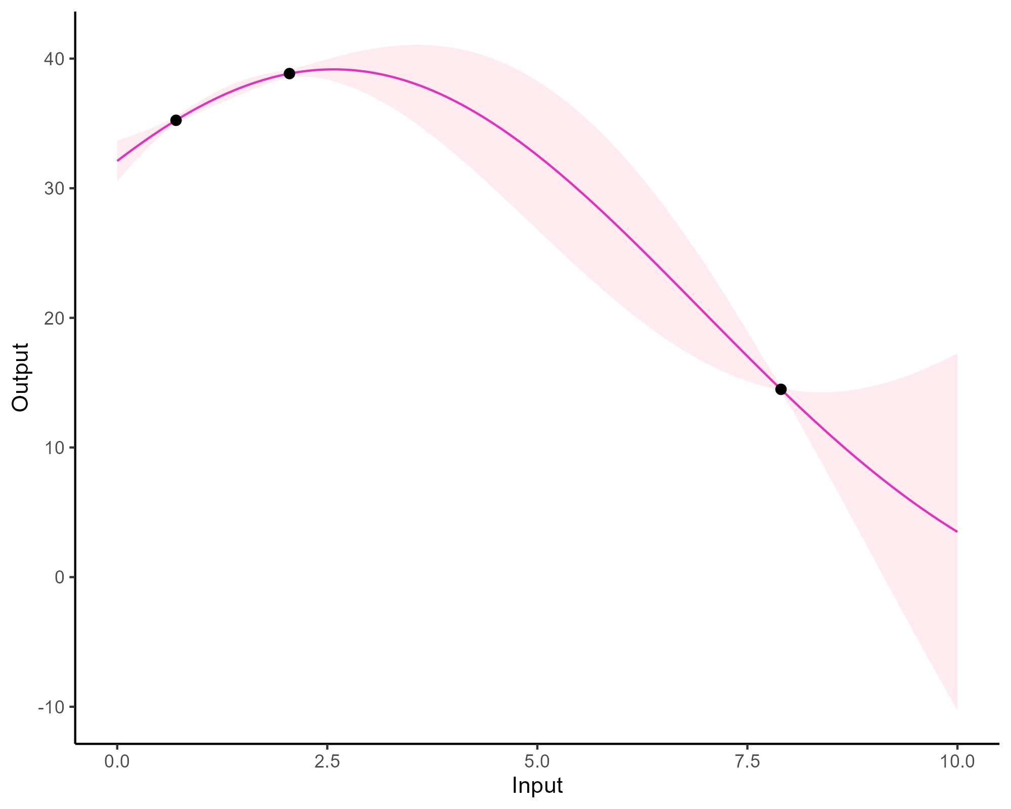
A quick one I promise

See, already done. Let the real fun begin!

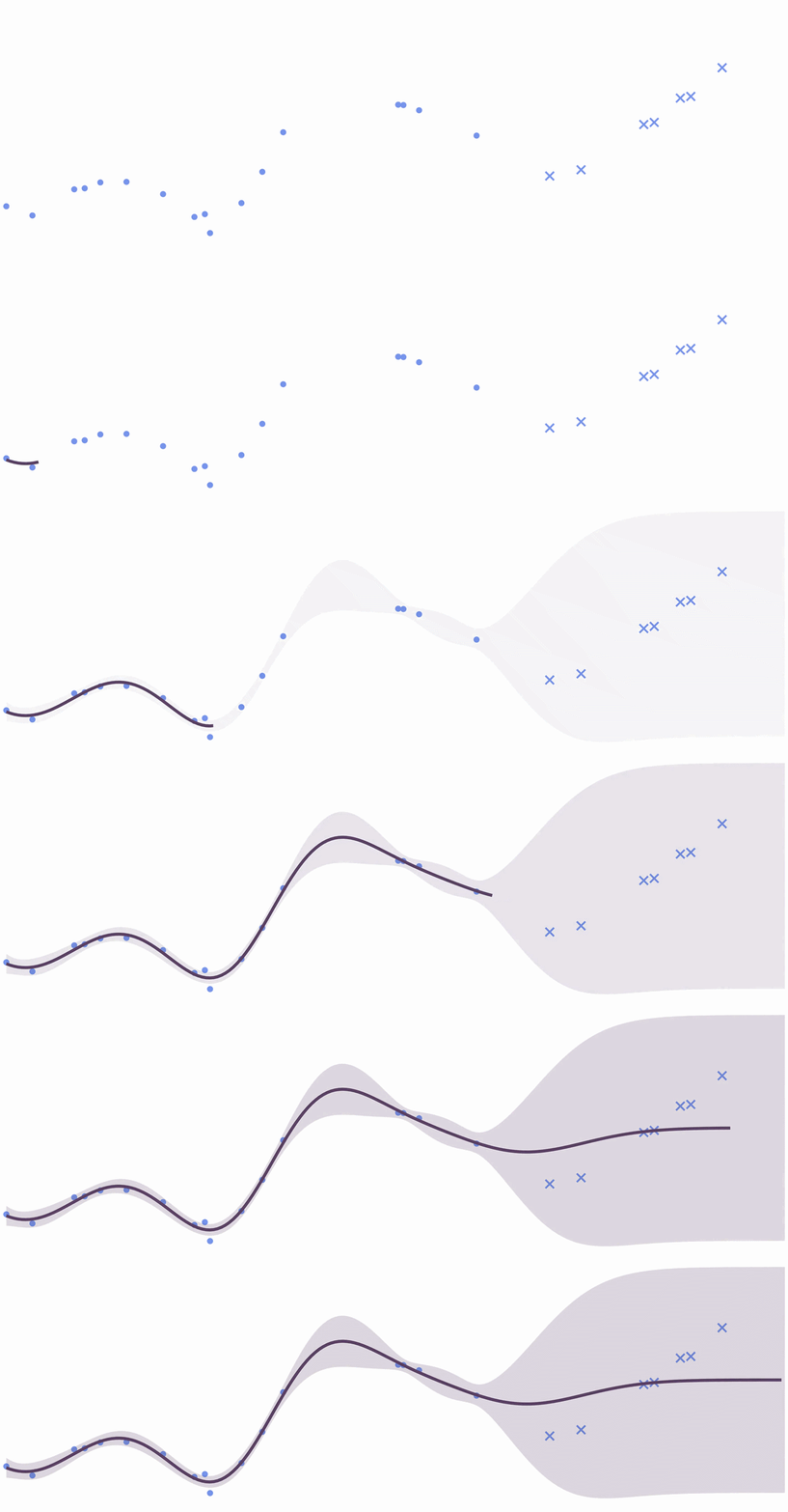
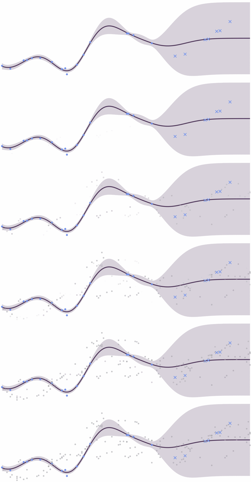
Forecasting with a unique GP

A long history of old and modern Multi-Output strategies

A large litterature in geostatistics, from the origins in the 60s, is known as co-kriging.
Alvarez et al. - Kernels for Vector-Valued Functions: A Review - Foundations and Trends in Machine Learning, 2011
Parra and Tobar - Spectral mixture kernels for multi-output Gaussian processes - NeurIPS, 2017
Liu et al. - Remarks on multi-output Gaussian process regression - Knowledge-Based Systems, 2018
Bruinsma et al. - Scalable Exact Inference in Multi-Output Gaussian Processes - PMLR, 2020
Van der Wilk et al. - A framework for interdomain and multioutput Gaussian processes - arXiv preprint, 2020

The following section is largely inspired from this talk (way more details here):

GPSS 2017 video recording - Multi-Output Gaussian Processes - Mauricio Alvarez

Multi-Output GPs: exploiting explicit correlations

Leveraging existing correlations across Outputs instead of multiple independent GPs.

Defining multi-output kernels, explicitly modelling correlations between each output-input couple. A classical assumption is separable covariance structures:

\[k\left((i, x),\left(j, x^{\prime}\right)\right)=\operatorname{cov}\left(f_i(x), f_j\left(x^{\prime}\right)\right)=K^{\mathrm{O}}_{i, j} \times k_{\mathrm{I}}\left(x, x^{\prime}\right)\]

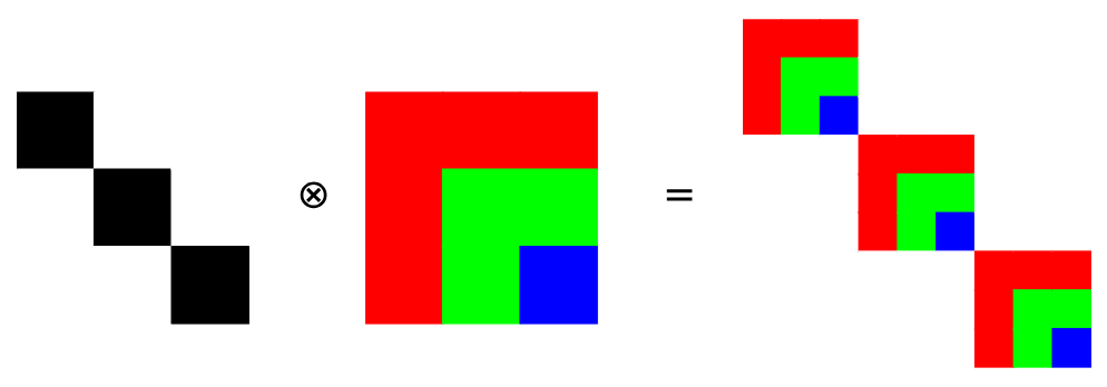
The Outputs are stacked into one vector, and the matrices built from those kernels can be represented through a Kronecker product \(\textbf{K} = \textbf{K}^{\mathrm{O}} \otimes \textbf{K}_{\mathrm{I}}\), such that

\[ \mathbf y = \begin{bmatrix} \mathbf y_1\\[-2pt] \vdots\\[-2pt] \mathbf y_O \end{bmatrix}, \qquad \mathbf y \sim \mathcal N\!\left( \mathbf m,\, \textbf{K}+\sigma^2 I \right).\]

GP inference and prediction procedures are similar to standard GPs, only the kernel changes.

Intuition behind the Kronecker formulation

Credits: Neil Lawrence

Multi-Output GPs: the ideal case

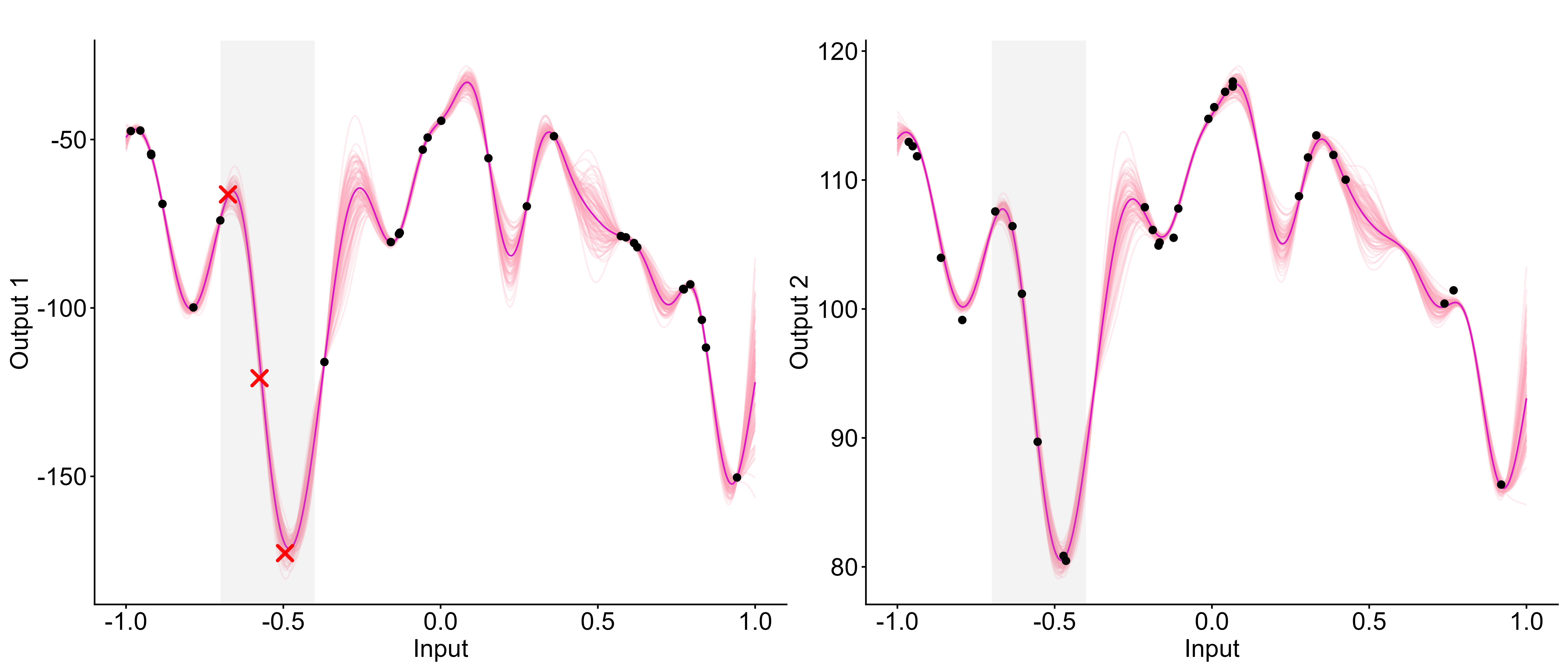
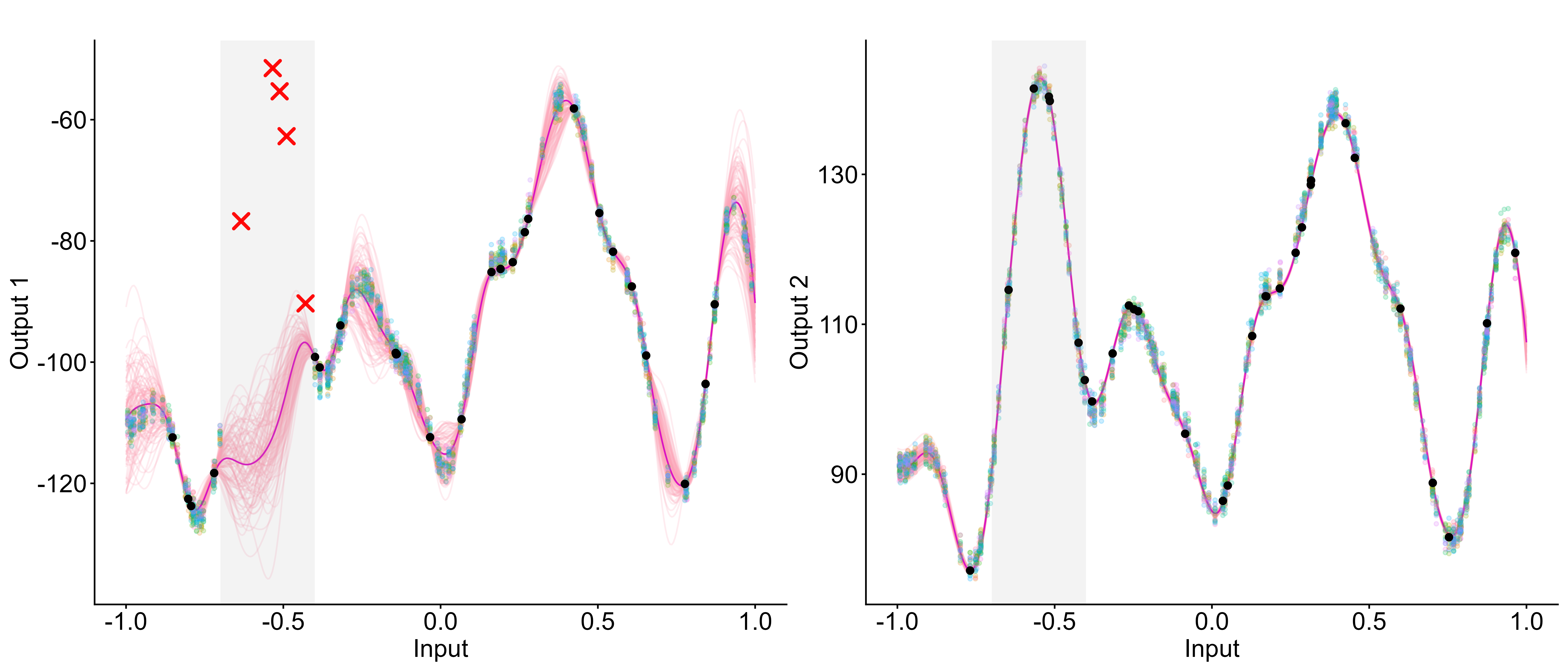
Multi-Output GPs thrive in interpolation problems, leveraging other Outputs to fill the gaps.

Intrinsic Corregionalisation Model (ICM)

A set of functions \(\{f_o(\mathbf{x})\}_{o=1}^O\) can be expressed through ICM as:

\[f_o(\mathbf{x}) = \sum_{i =1}^Ra_{o}^{i}u^{i}(\mathbf{x}),\]

where the functions \(u^{i}(\mathbf{x})\) are independent GPs with shared covariance kernel \(k(\mathbf{x}, \mathbf{x}')\).

For \(\textbf{f}(\mathbf{x}) = [f_1(\mathbf{x}) \cdots f_O(\mathbf{x})]^{\top}\), the covariance \(cov[\textbf{f}(\mathbf{x}), \textbf{f}(\mathbf{x}')]\) is defined as:

\[cov[\textbf{f}(\mathbf{x}), \textbf{f}(\mathbf{x}')] = \textbf{A}\textbf{A}^\top\,k(\mathbf{x}, \mathbf{x}') = \textbf{B}\,k(\mathbf{x}, \mathbf{x}'),\]

where \(\textbf{A} = [\mathbf{a}^1 \; \mathbf{a}^2 \cdots \mathbf{a}^R]\). The rank of \(\textbf{B}\in\mathbb{R}^{O\times O}\) depends on the value of \(R\).

If the Outputs are considered noise-free, ICM predictions are equivalent to independent ones.

Linear Model of Corregionalisation (LMC)

\[f_d(\mathbf{x}) = \sum_{q =1}^Q\sum_{i=1}^{R_q} a^i_{d,q}u^i_{q}(\mathbf{x}),\]

In an LMC, there are \(Q\) groups of \(R_q\) independent GPs. Those underlying GPs share identical group-specific covariance structures \(k_{q}(\mathbf{x},\mathbf{x}')\).

\[cov[\textbf{f}(\mathbf{x}), \textbf{f}(\mathbf{x}')] = \sum_{q=1}^Q \textbf{A}_q\textbf{A}_q^\top\,k_q(\mathbf{x}, \mathbf{x}') = \sum_{q=1}^Q\textbf{B}_q\,k_q(\mathbf{x}, \mathbf{x}'),\]

where \(\textbf{A}_q = [\mathbf{a}^1_q \; \mathbf{a}^2_q \cdots \mathbf{a}^{R_q}_q]\) and the rank of each \(\textbf{B}_q\) is now \(R_q\).

The matrices \(\textbf{B}_q\) are known as the coregionalisation matrices and allow non-trivial interractions across Outputs by exploiting explicit inter-output covariance elements learned from data.

Process Convolution (PC)

PC defines functions through a convolution integral between a smooting kernel and a latent GP:

\[f_d(\mathbf{x}) = \int_{\mathcal{X}} G_{d}(\mathbf{x}-\mathbf{z})u(\mathbf{z})\mathop{}\!\mathrm{d}\mathbf{z} = G_{d}(\mathbf{x})\ast u(\mathbf{x}).\]

Although this integral is intractable in general, specific Gaussian forms for kernels lead to

\[cov\left[f_d(\mathbf{x}),f_{d'}(\mathbf{x'})\right] = \frac{S_{d}S_{d'}}{(2\pi)^{p/2}|\Sigma|^{1/2}} \exp\left[-\frac{1}{2}\left(\mathbf{x}-\mathbf{x}'\right)^{\top} \Sigma^{-1}\left(\mathbf{x}-\mathbf{x}'\right)\right],\] with \(\ \ \ \Sigma = P_{d}^{-1}+P_{d'}^{-1} + \Lambda^{-1}\)

Many Multi-Ouput GPs models can actually be written as particular cases of more a general form

\[f_d(\mathbf{x}) = \sum_{q=1}^Q\sum_{i=1}^{R_q}\int_{\mathcal{X}} G^i_{d,q}(\mathbf{x}-\mathbf{z})u^i_q(\mathbf{z})\mathop{}\!\mathrm{d}\mathbf{z},\]

for specific choices of \(Q\), \(R_q\) and associated smoothing kernels \(G^i_{d,q}\) (typically through a Dirac).

Generative flexibility

Some limits of Multi-Output GPs

Natively, the computational complexity for exact training is \(\mathcal{O}(\color{red}{O}^3N^3)\),
In practice, training the inter-task correlations (\(\textbf{K}^{\mathrm{O}}\)) can be tricky and unstable,
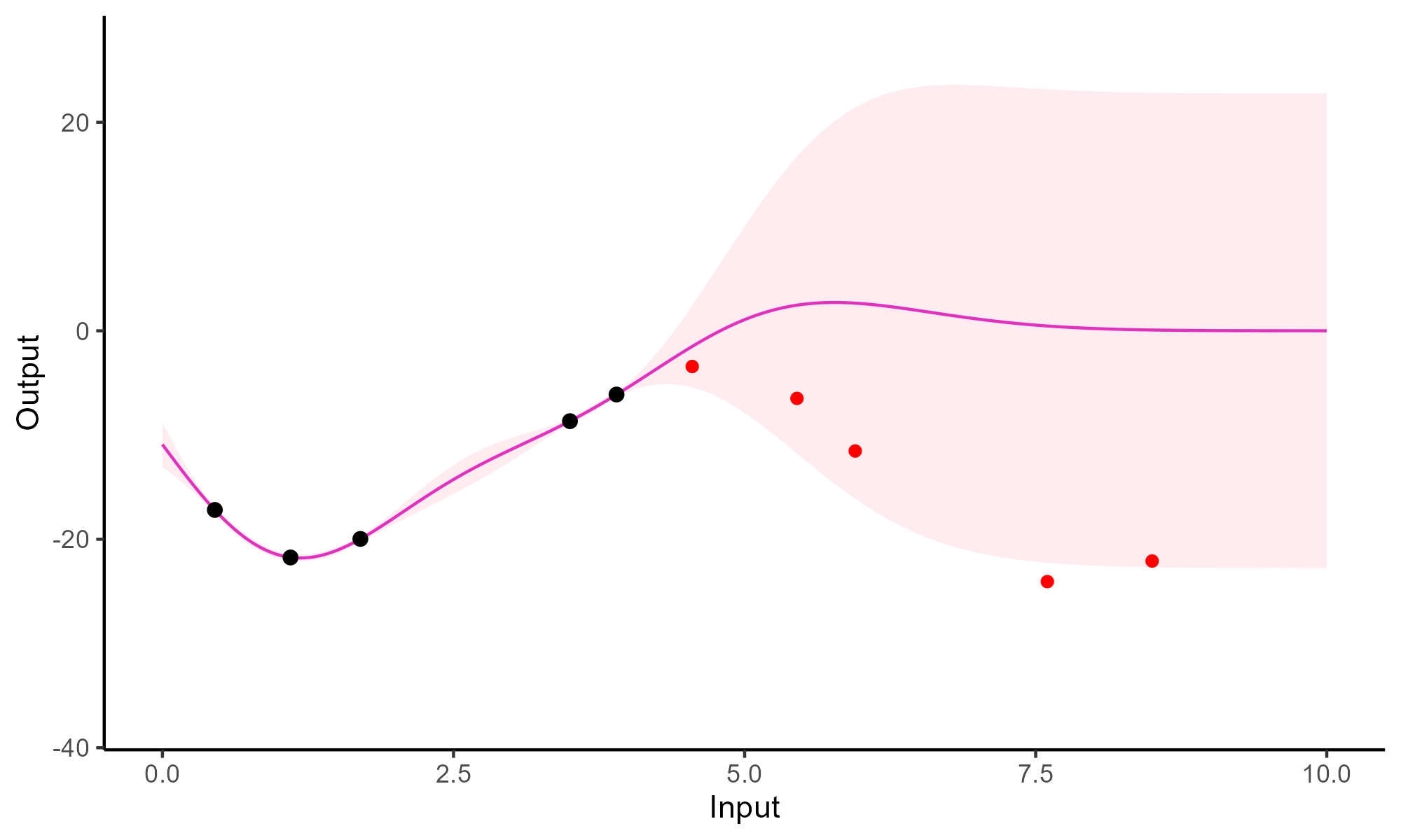
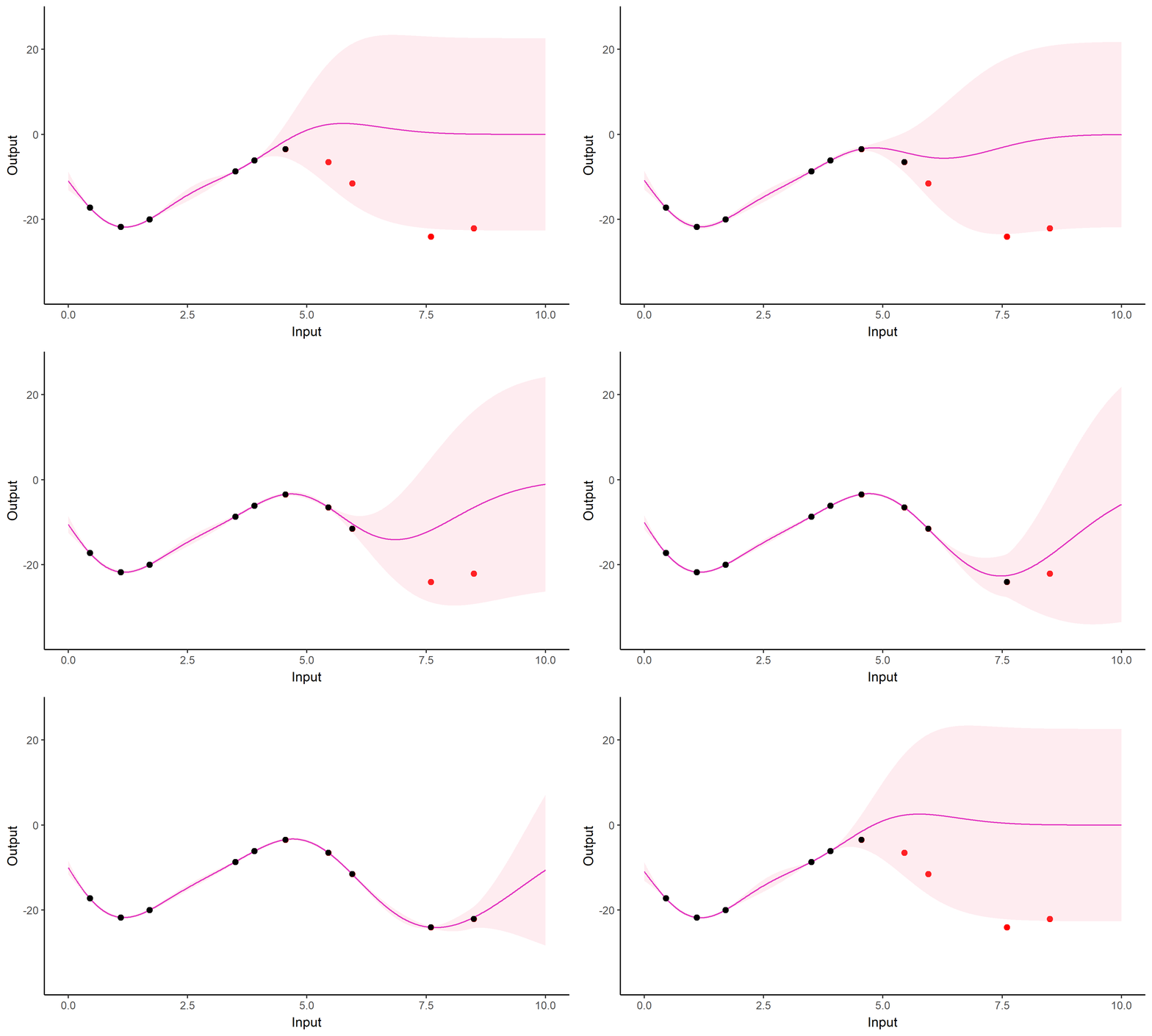
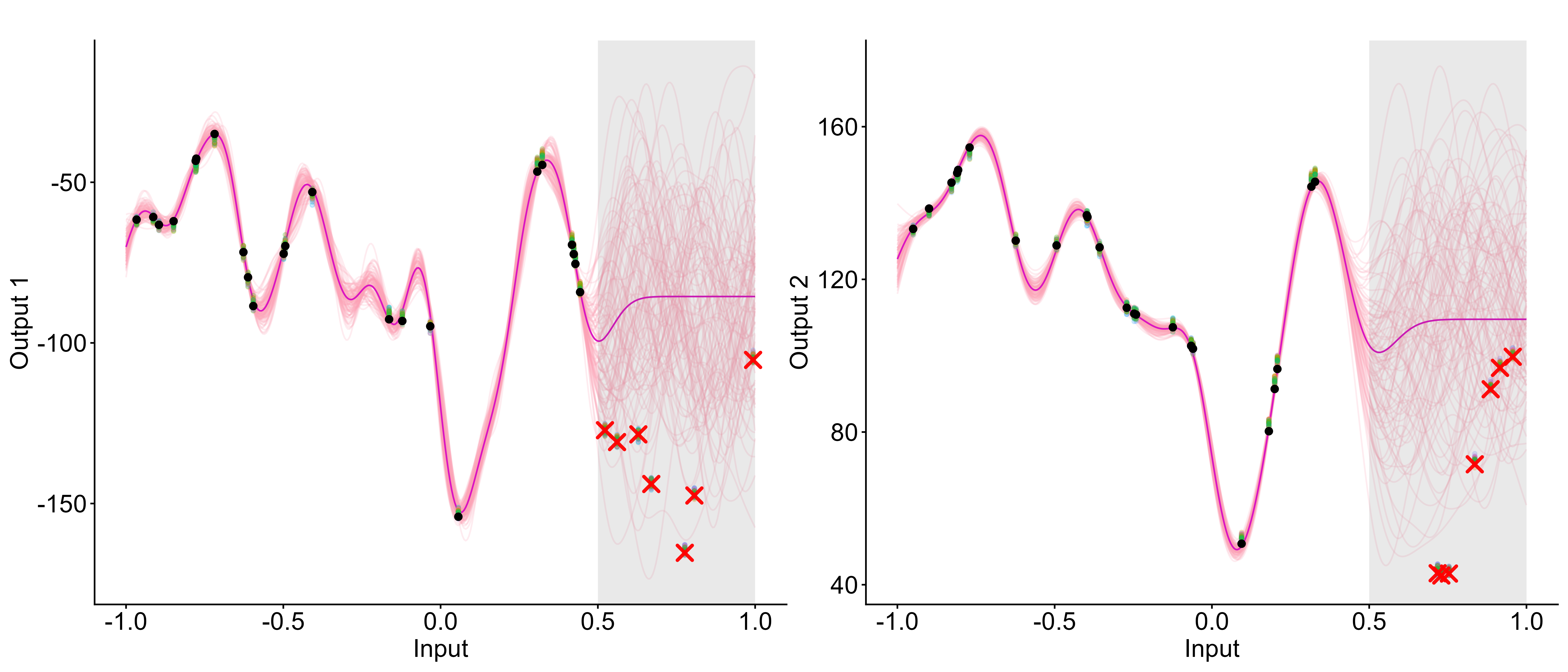
Poor performance on intervals unobserved for all Outputs (e.g. forecasting).

Another paradigm: Multi-Task GPs with shared mean process

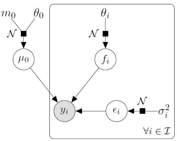
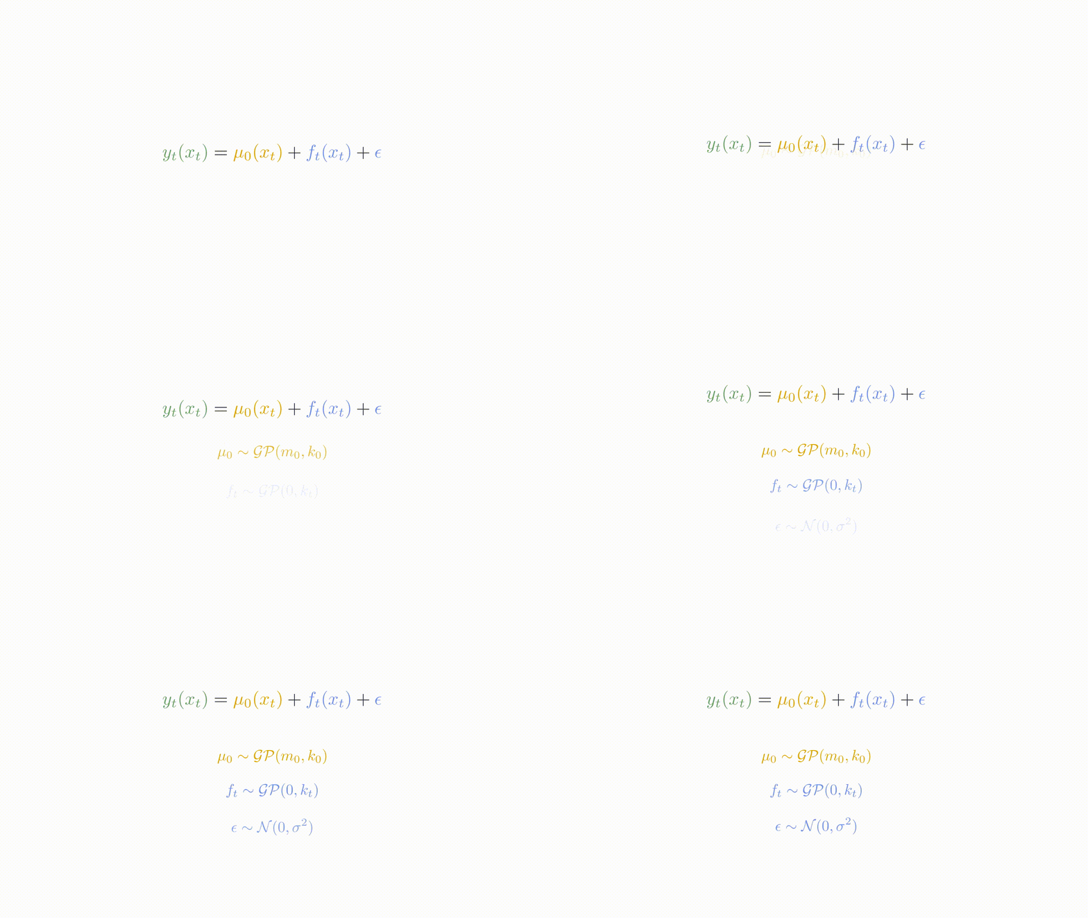
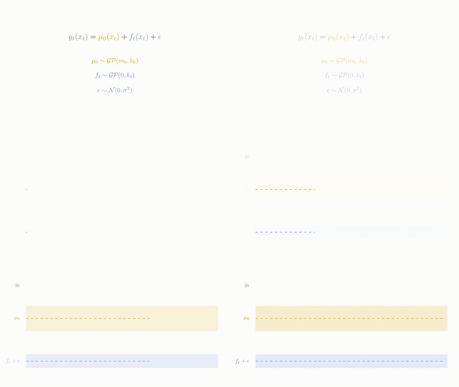
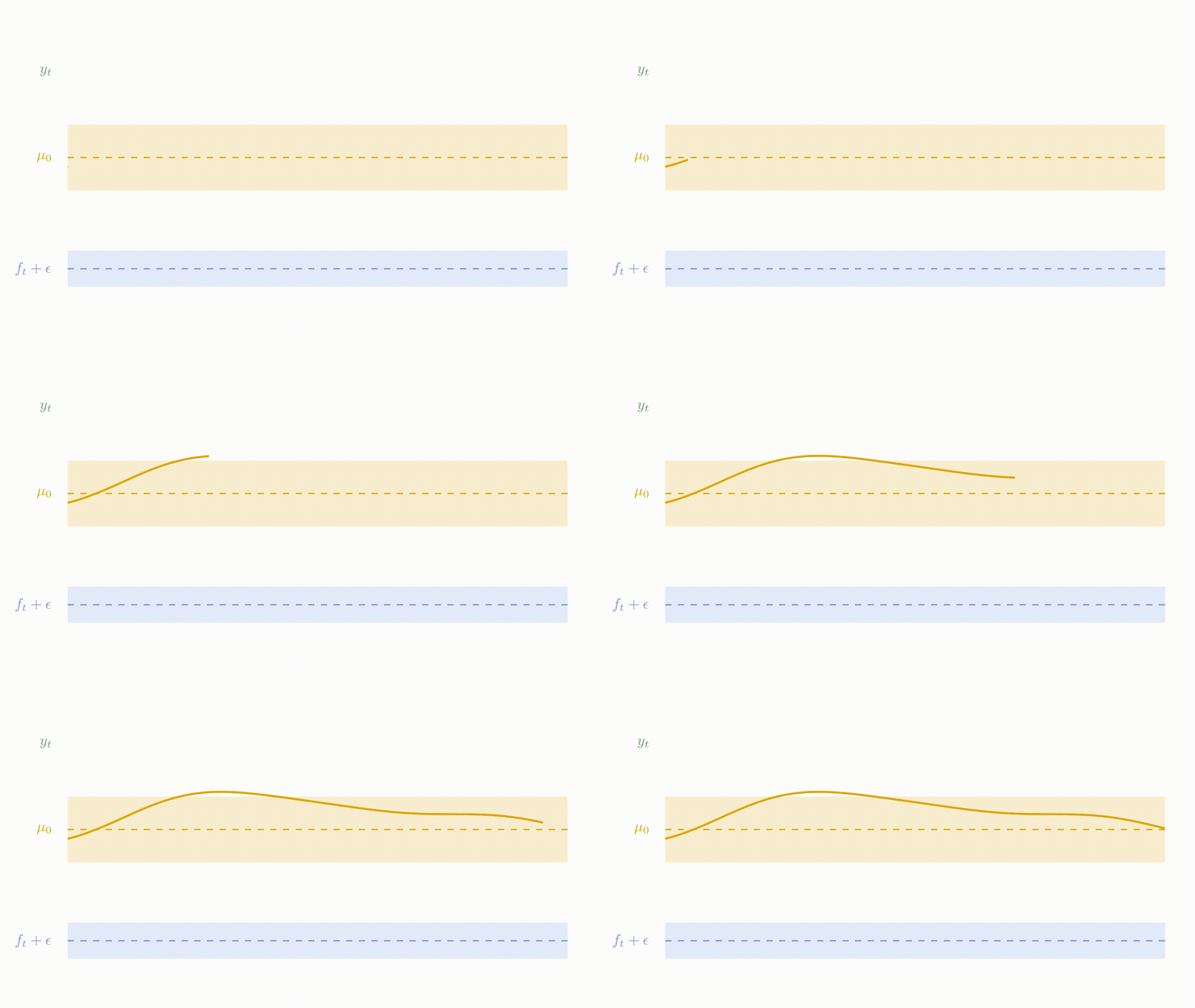
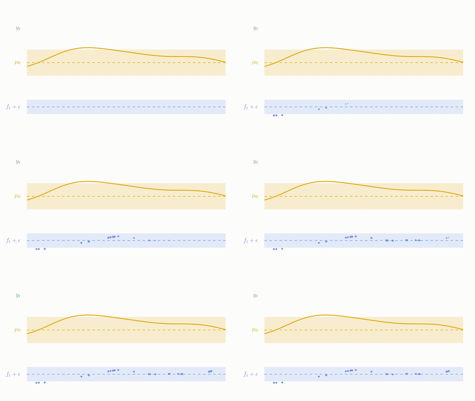
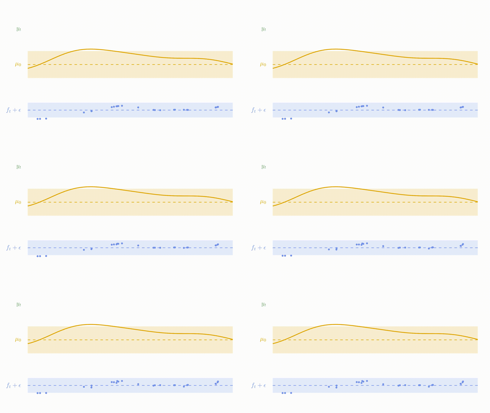
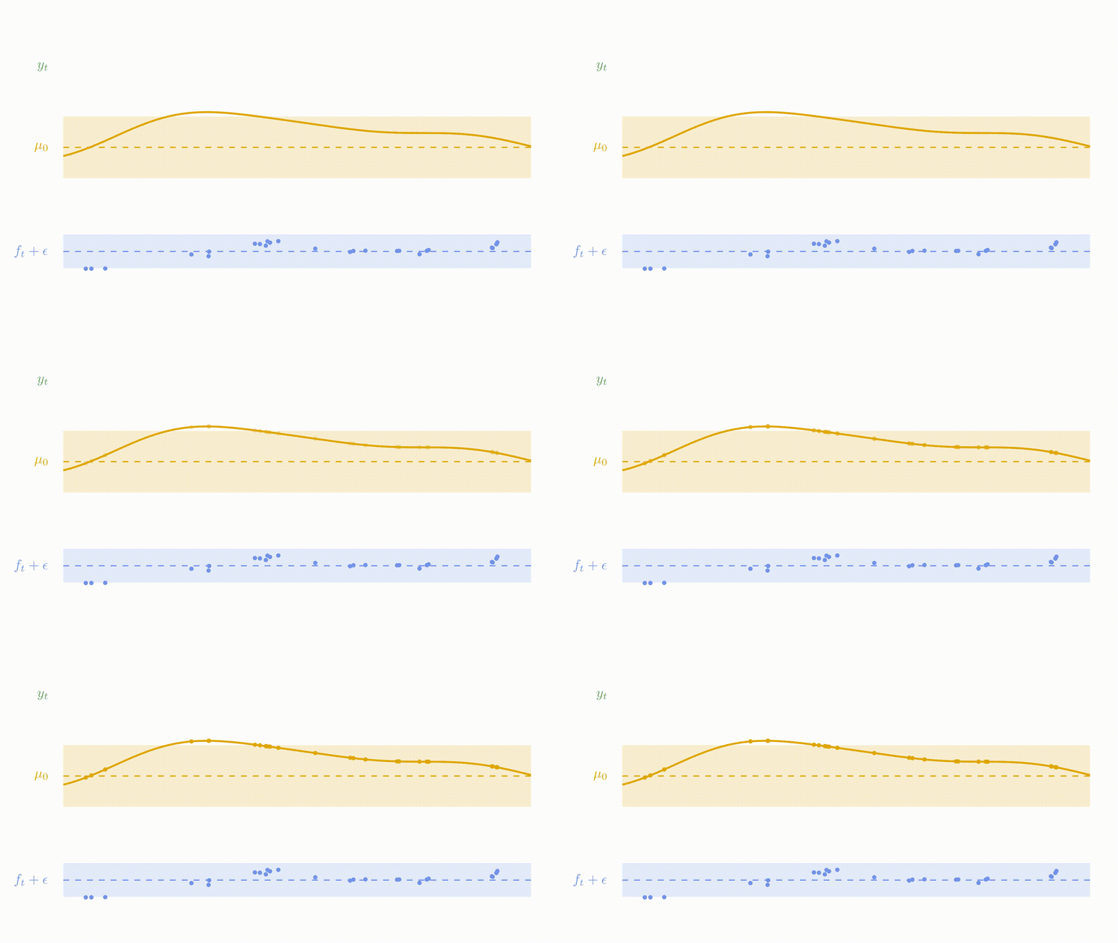
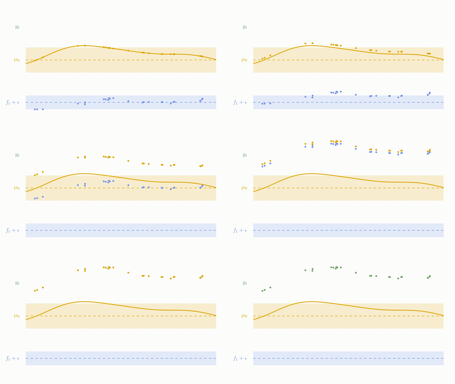
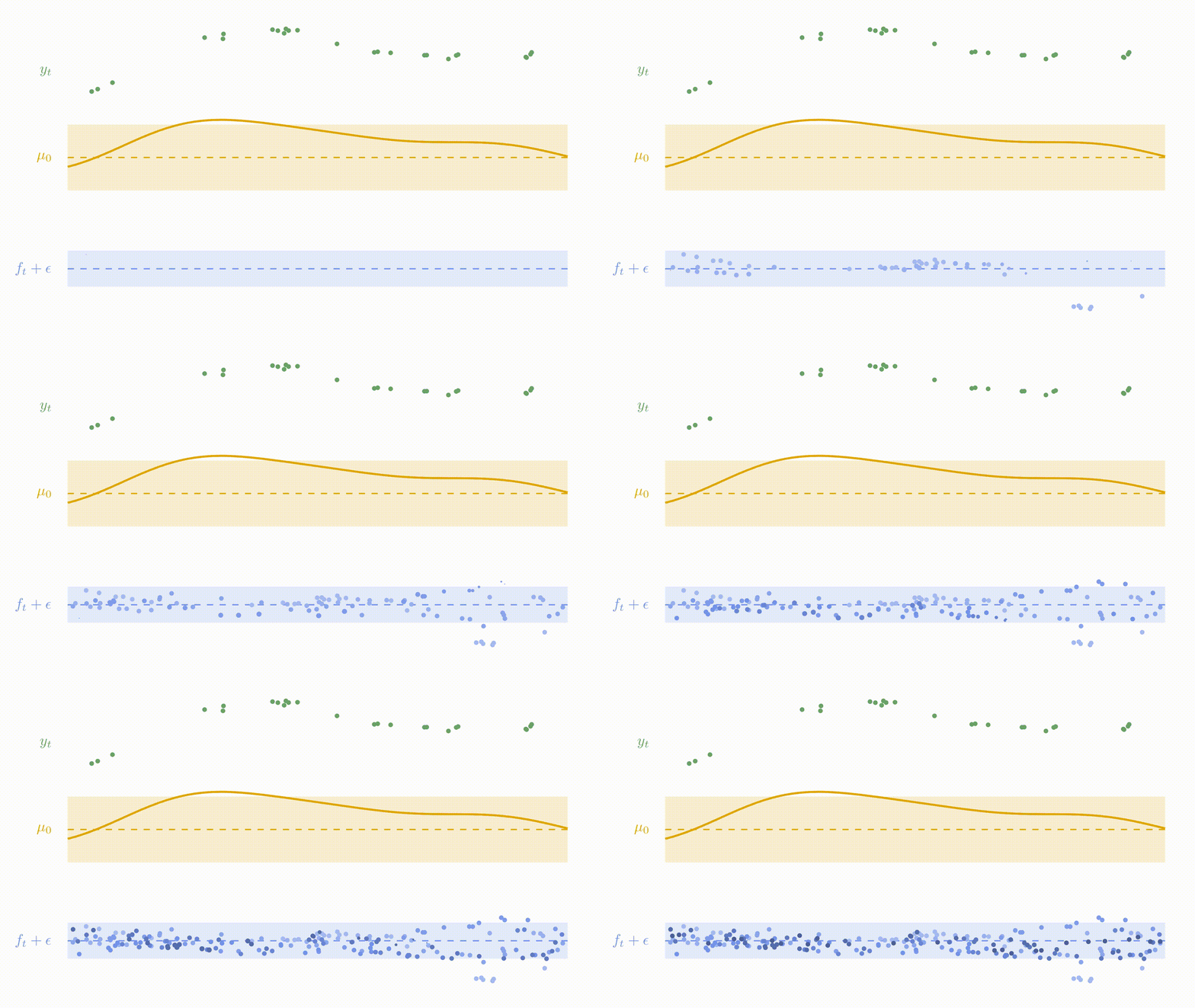
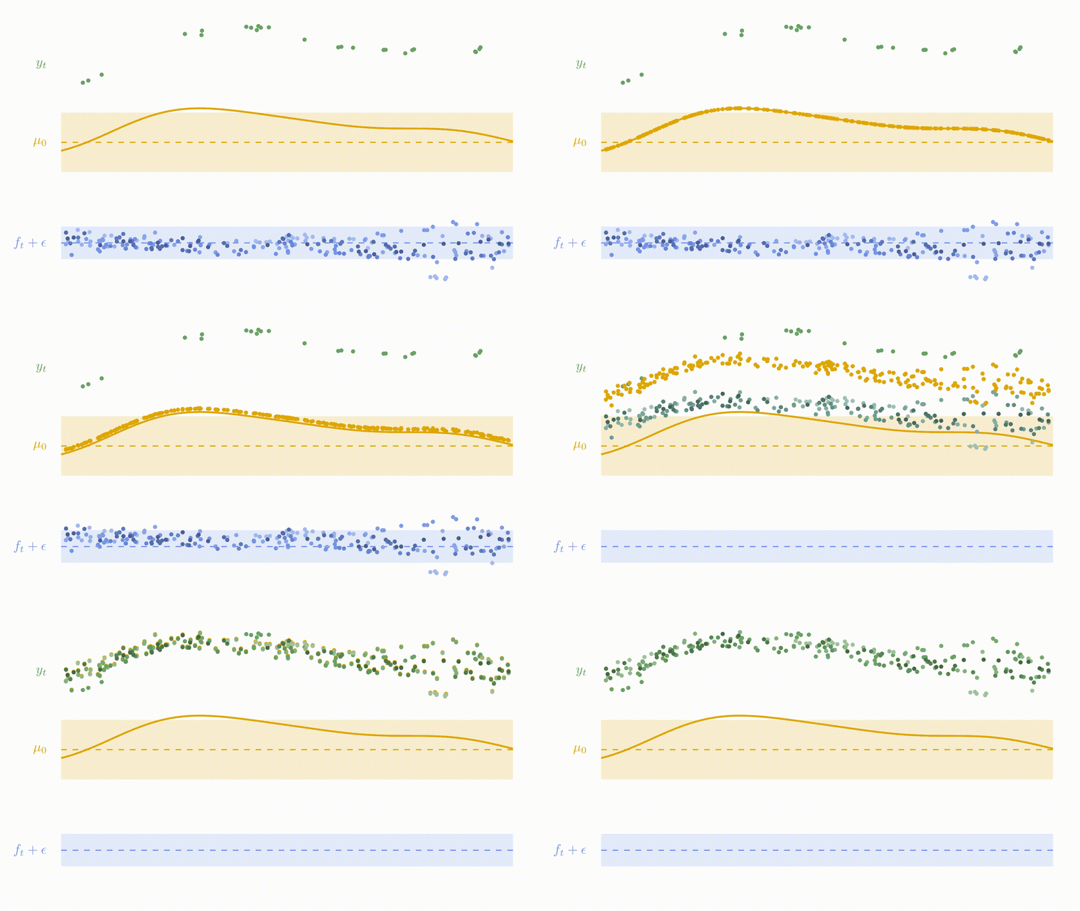
\[y_t = \mu_0 + f_t + \epsilon_t, \hspace{3cm} \forall t = 1, \dots, T\]

with:

\(\mu_0 \sim \mathcal{GP}(m_0, K_{0}),\)
\(f_t \sim \mathcal{GP}(0, \Sigma_{\theta_t}), \ \perp \!\!\! \perp_t,\)
\(\epsilon_t \sim \mathcal{GP}(0, \sigma_t^2), \ \perp \!\!\! \perp_t.\)

It follows that:

\[y_t \mid \mu_0 \sim \mathcal{GP}(\mu_0, \Sigma_{\theta_t} + \sigma_t^2 I), \ \perp \!\!\! \perp_t\]

\(\rightarrow\) Unified GP framework with a shared mean process \(\mu_0\), and task-specific process \(f_t\),
\(\rightarrow\) Naturaly handles irregular grids of input data.

Goal: Learn the hyper-parameters, (and \(\mu_0\)’s hyper-posterior).
Difficulty: The likelihood depends on \(\mu_0\), and tasks are not independent.

Generative modelling assumptions

Generative modelling assumptions

EM algorithm

E-step

\[ \begin{align} p(\mu_0(\color{grey}{\mathbf{x}}) \mid \textbf{y}, \hat{\Theta}) &\propto \mathcal{N}(\mu_0(\color{grey}{\mathbf{x}}); m_0(\color{grey}{\textbf{x}}), \textbf{K}_{0}^{\color{grey}{\textbf{x}}}) \times \prod\limits_{t =1}^T \mathcal{N}(\mathbf{y}_t; \mu_0( \color{purple}{\textbf{x}_i}), \boldsymbol{\Psi}_{\hat{\theta}_i, \hat{\sigma}_i^2}^{\color{purple}{\textbf{x}_i}}) \\ &= \mathcal{N}(\mu_0(\color{grey}{\mathbf{x}}); \hat{m}_0(\color{grey}{\textbf{x}}), \hat{\textbf{K}}^{\color{grey}{\textbf{x}}}), \end{align} \]

\(\hat{\textbf{K}}^{\color{grey}{\textbf{x}}} = ({\textbf{K}_{0}^{\color{grey}{\textbf{x}}}}^{-1} + \sum\limits_{t = 1}^T {\boldsymbol{\Psi}_{\hat{\theta}_i, \hat{\sigma}_i^2}^{\color{purple}{\textbf{x}_i}}}^{-1})^{-1}\)
\(\hat{m}_0(\color{grey}{\textbf{x}}) = \hat{\textbf{K}}^{\color{grey}{\textbf{x}}}({\textbf{K}_{0}^{\color{grey}{\textbf{x}}}}^{-1} m_0(\color{grey}{\mathbf{x}}) + \sum\limits_{t = 1}^T {\boldsymbol{\Psi}_{\hat{\theta}_i, \hat{\sigma}_i^2}^{\color{purple}{\textbf{x}_i}}}^{-1} \mathbf{y}_t)\).

M-step

\[ \begin{align*} \hat{\Theta} &= \underset{\Theta}{\arg\max} \ \ \sum\limits_{t = 1}^{T}\left\{ \log \mathcal{N} \left( \mathbf{y}_t; \hat{m}_0(\color{purple}{\mathbf{x}_t}), \boldsymbol{\Psi}_{\theta_t, \sigma^2}^{\color{purple}{\mathbf{x}_t}} \right) - \dfrac{1}{2} Tr \left( \hat{\mathbf{K}}^{\color{purple}{\mathbf{x}_t}} {\boldsymbol{\Psi}_{\theta_t, \sigma^2}^{\color{purple}{\mathbf{x}_t}}}^{-1} \right) \right\}. \end{align*} \]

Covariance structure assumption and computational complexity

Sharing the covariance structures or not offers a compromise between flexibility and parsimony:

One optimisation problem for \(\theta\), and a shared process for all tasks,
\(\color{blue}{T}\) distinct optimisation problems for \(\{\theta_t\}_t\), and task-specific processes.

Major interests:

Both approaches scale linearly with the number of tasks,
Parallel computing can be used to speed up training.

Overall, the computational complexity is: \[ \mathcal{O}(\color{blue}{T} \times N_t^3 + N^3) \]

with \(N = \bigcup\limits_{t = 1}^\color{blue}{T} N_t\)

Prediction

For a new task \(*\), we want to make predictions on-the-flow from its data \(\{\textbf{x}_*, y_*\}\). Let us recall:

\[y_* \mid \mu_0 \sim \mathcal{GP}(\mu_0, \boldsymbol{\Psi}_{\theta_*, \sigma_*^2}), \ \perp \!\!\! \perp_t\]

Information about training tasks is stored in the hyperposterior distribution \(p(\mu_0(\color{grey}{\mathbf{x}}) \mid \textbf{y})\).

How to derive an analytical predictive distribution at arbitrary inputs \(\mathbf{x}^{p}\)?

Prediction: the key idea

Defining a multi-task prior distribution by:

conditioning on training data,
integrating over \(\mu_0\)’s hyper-posterior distribution.

\[\begin{align} p(y_* (\textbf{x}_*^{p}) \mid \textbf{y}) &= \int p\left(y_* (\textbf{x}_*^{p}) \mid \textbf{y}, \mu_0(\textbf{x}_*^{p})\right) p(\mu_0 (\textbf{x}_*^{p}) \mid \textbf{y}) \ d \mu_0(\mathbf{x}^{p}_{*}) \\ &= \int \underbrace{ p \left(y_* (\textbf{x}_*^{p}) \mid \mu_0 (\textbf{x}_*^{p}) \right)}_{\mathcal{N}(y_*; \mu_0, \Psi_*)} \ \underbrace{p(\mu_0 (\textbf{x}_*^{p}) \mid \textbf{y})}_{\mathcal{N}(\mu_0; \hat{m}_0, \hat{K})} \ d \mu_0(\mathbf{x}^{p}_{*}) \\ &= \mathcal{N}( \hat{m}_0 (\mathbf{x}^{p}_{*}), \underbrace{\Psi_* + \hat{K}}_{\Gamma}) \end{align}\]

Final prediction: the good old GP formula

Multi-Task prior:

\[p \left( \begin{bmatrix} y_*(\color{grey}{\mathbf{x}_{*}}) \\ y_*(\color{purple}{\mathbf{x}^{p}}) \\ \end{bmatrix} \mid \textbf{y} \right) = \mathcal{N} \left( \begin{bmatrix} y_*(\color{grey}{\mathbf{x}_{*}}) \\ y_*(\color{purple}{\mathbf{x}^{p}}) \\ \end{bmatrix}; \ \begin{bmatrix} \hat{m}_0(\color{grey}{\mathbf{x}_{*}}) \\ \hat{m}_0(\color{purple}{\mathbf{x}^{p}}) \\ \end{bmatrix}, \begin{pmatrix} \Gamma_{\color{grey}{**}} & \Gamma_{\color{grey}{*}\color{purple}{p}} \\ \Gamma_{\color{purple}{p}\color{grey}{*}} & \Gamma_{\color{purple}{pp}} \end{pmatrix} \right)\]

Multi-Task posterior:

\[p(y_*(\color{purple}{\mathbf{x}^{p}}) \mid y_*(\color{grey}{\mathbf{x}_{*}}), \textbf{y}) = \mathcal{N} \Big( y_*(\color{purple}{\mathbf{x}^{p}}); \ \hat{\mu}_{*}(\color{purple}{\mathbf{x}^{p}}) , \hat{\Gamma}_{\color{purple}{pp}} \Big)\]

with:

\(\hat{\mu}_{*}(\color{purple}{\mathbf{x}^{p}}) = \hat{m}_0(\color{purple}{\mathbf{x}^{p}}) + \Gamma_{\color{purple}{p}\color{grey}{*}}\Gamma_{\color{grey}{**}}^{-1} (y_*(\color{grey}{\mathbf{x}_{*}}) - \hat{m}_0 (\color{grey}{\mathbf{x}_{*}}))\)
\(\hat{\Gamma}_{\color{purple}{pp}} = \Gamma_{\color{purple}{pp}} - \Gamma_{\color{purple}{p}\color{grey}{*}}\Gamma_{\color{grey}{**}}^{-1} \Gamma_{\color{grey}{*}\color{purple}{p}}\)

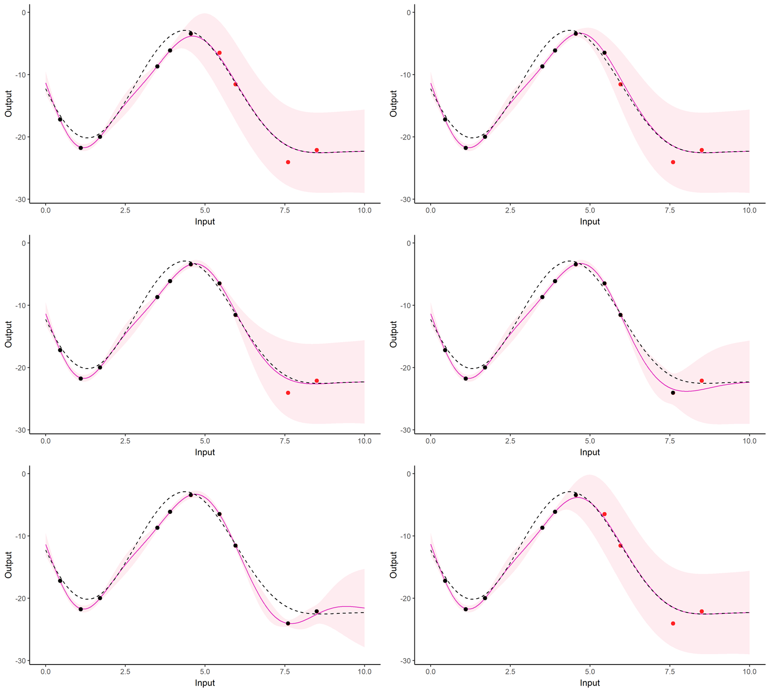
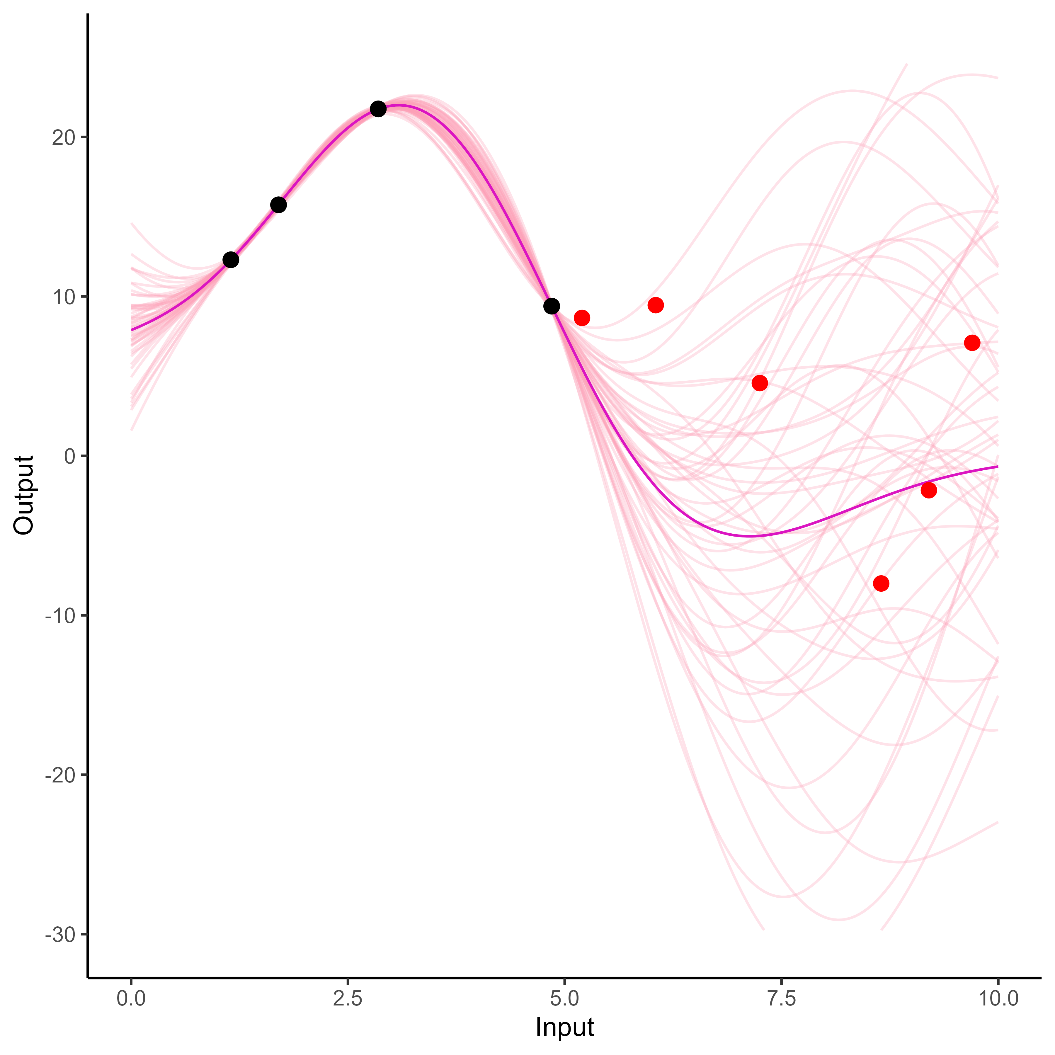
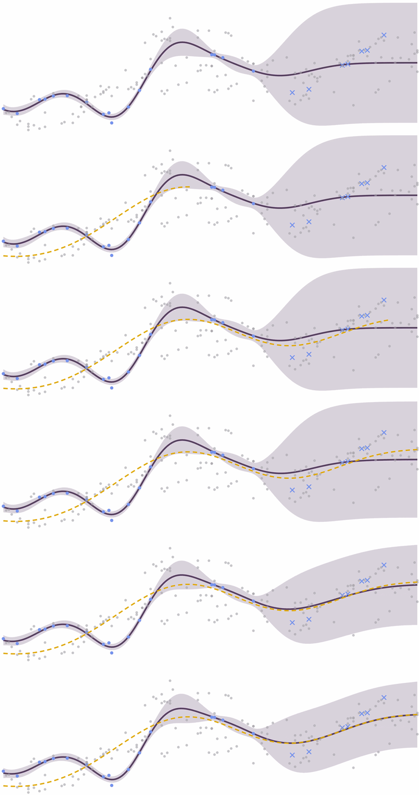
A GIF is worth a thousand words

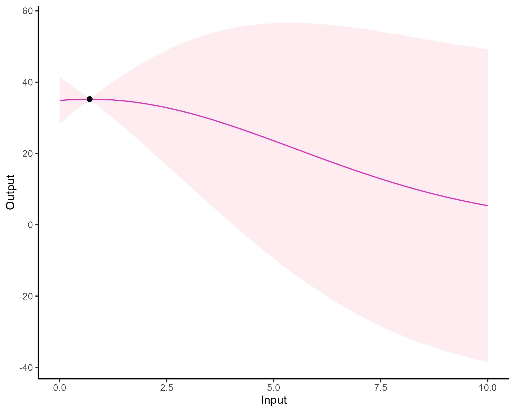
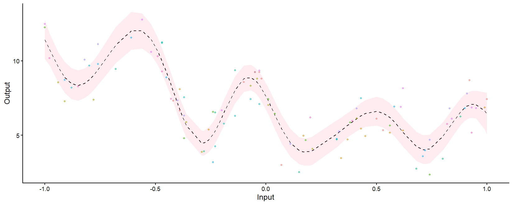
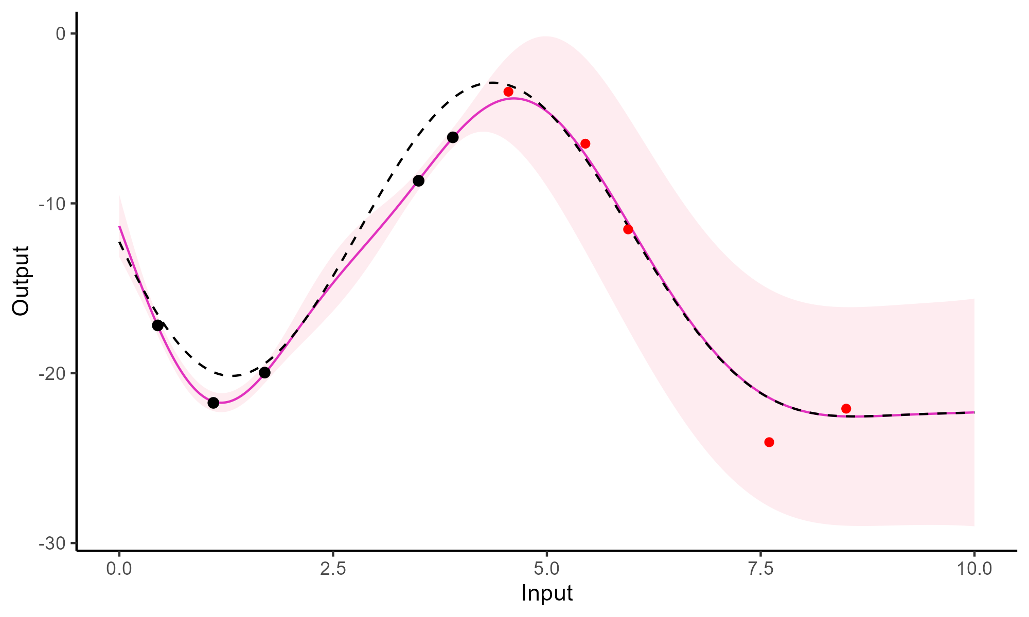
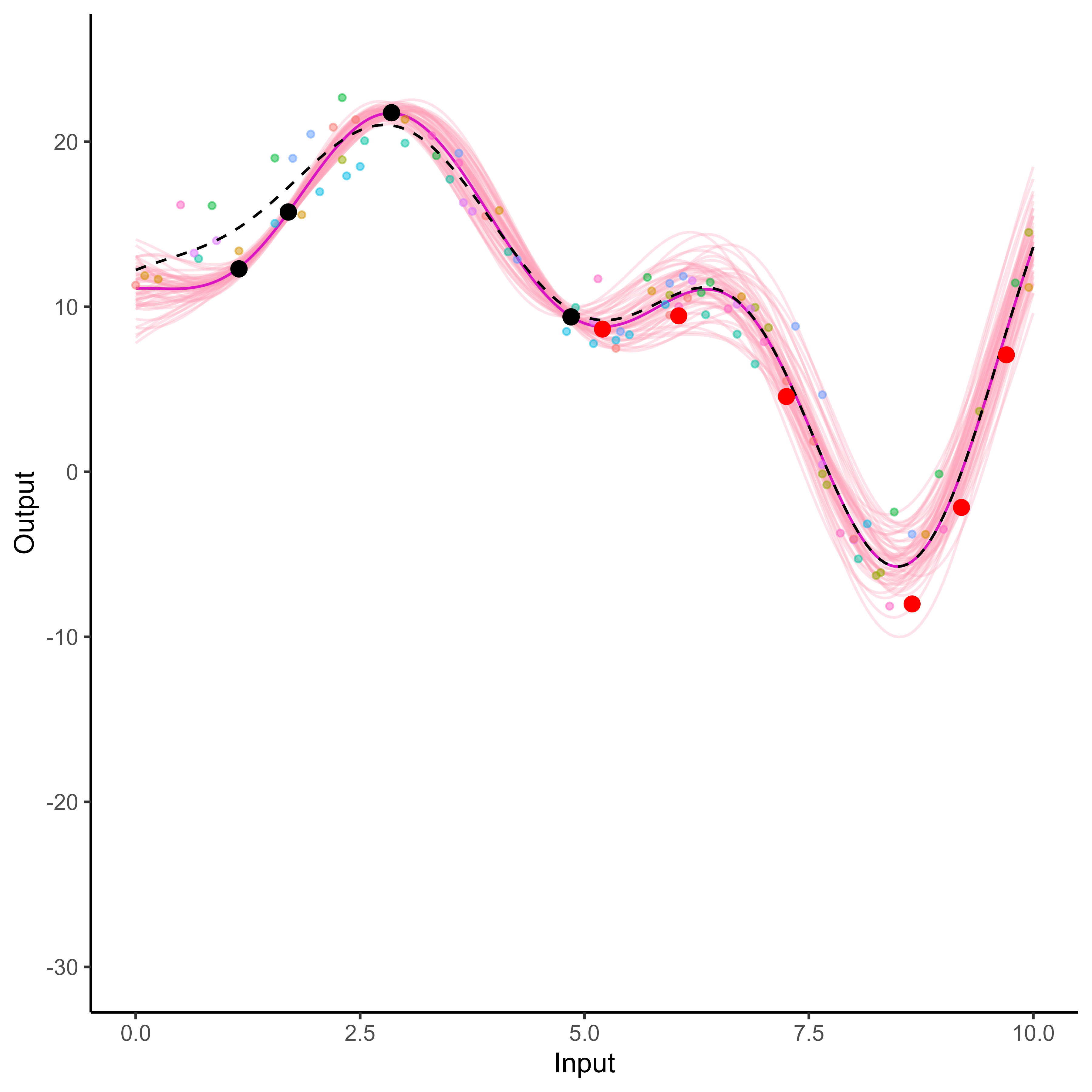
Comparison with single GP regression

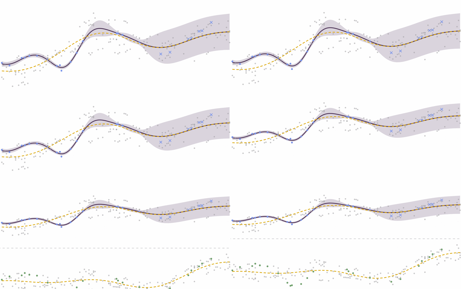
What happens with multi-dimensional inputs?

Yet another comparison with single GP regression

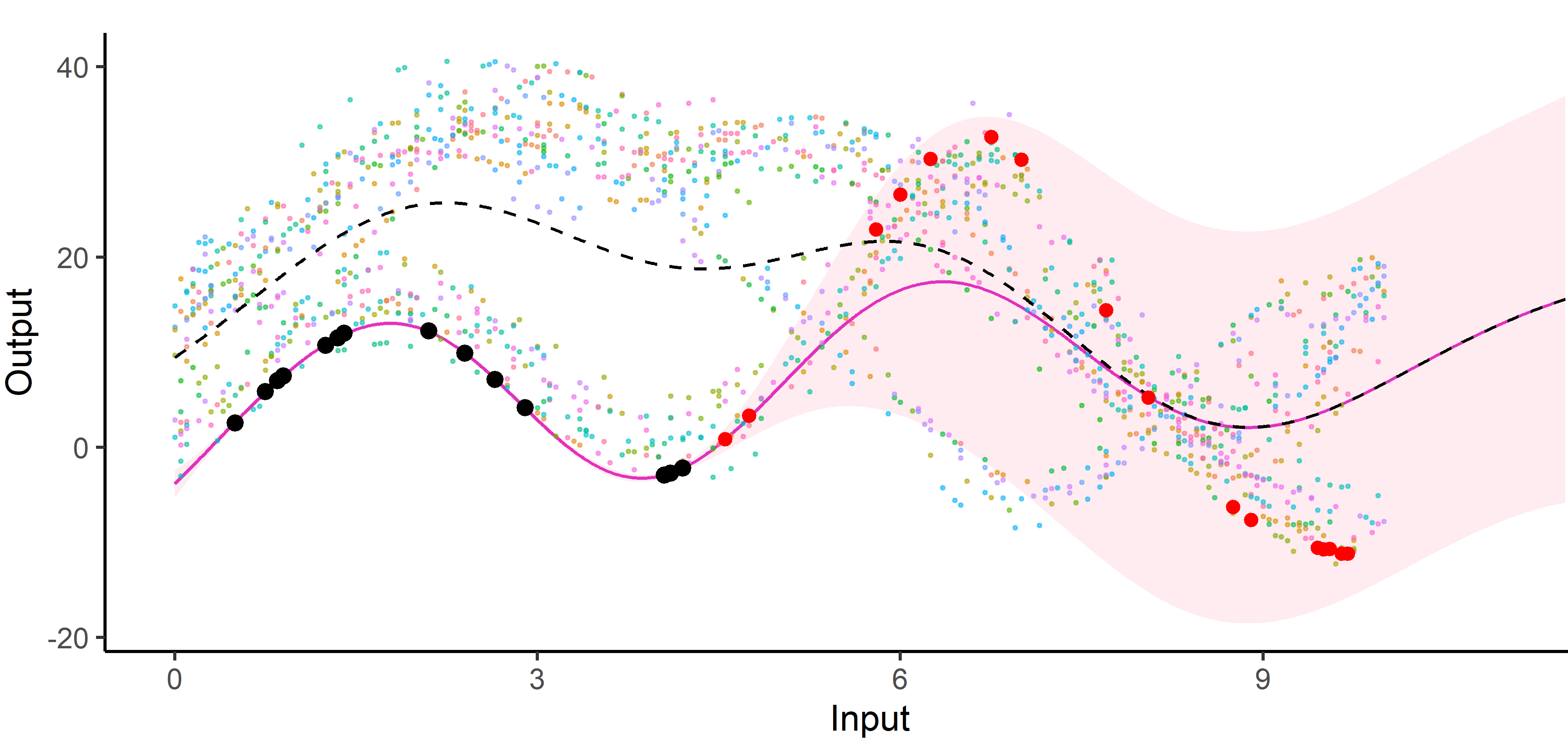
Multi-Task GPs regression provides more reliable predictions when individual processes are sparsely observed, while greatly reducing the associated uncertainty

Some limits of Multi-Task GPs

Does not capture cross-correlations between distinct phenomena, variables of interest,
A unique underlying mean process might be too restrictive,
Poor performance on intervals unobserved for all Tasks.

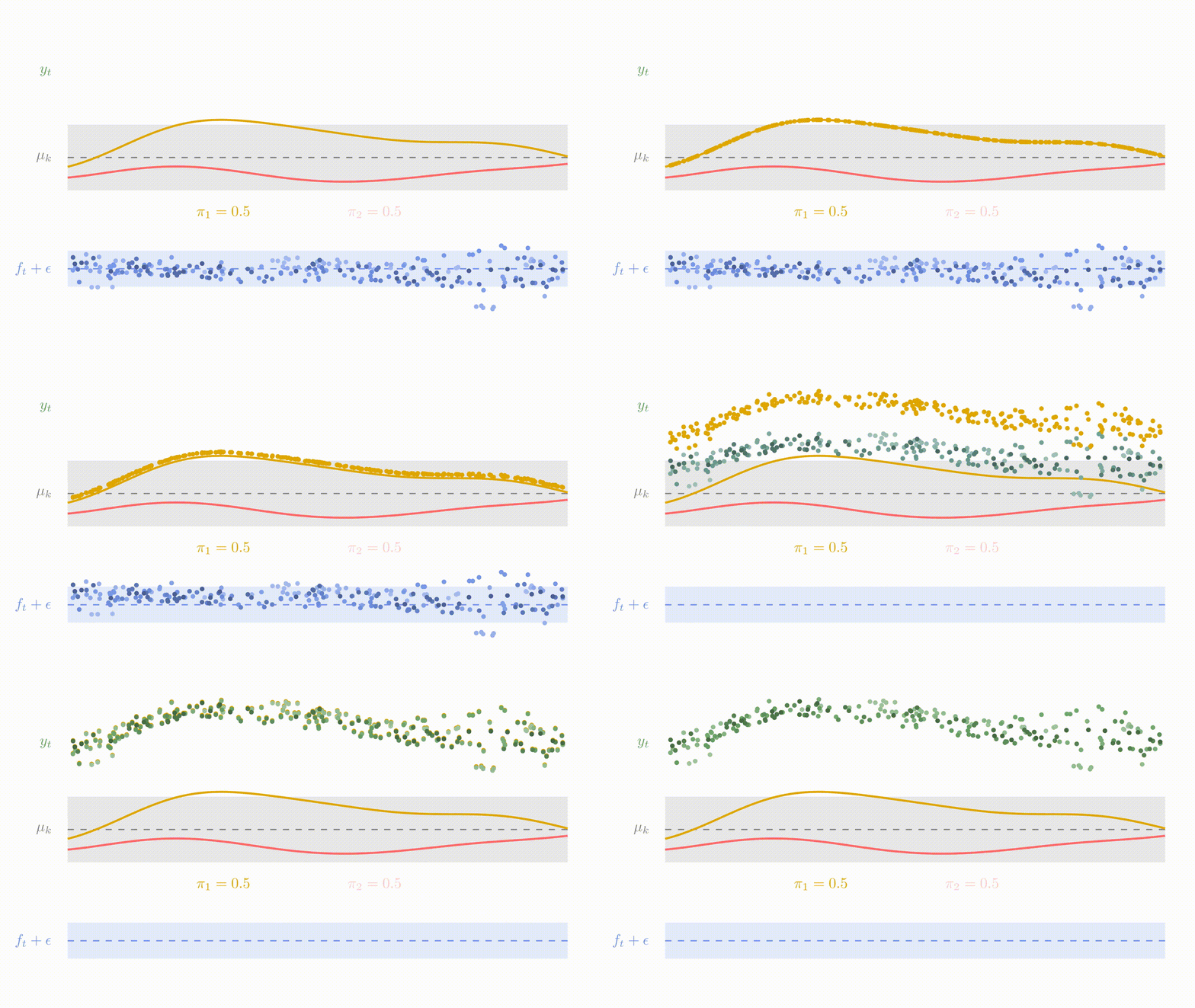
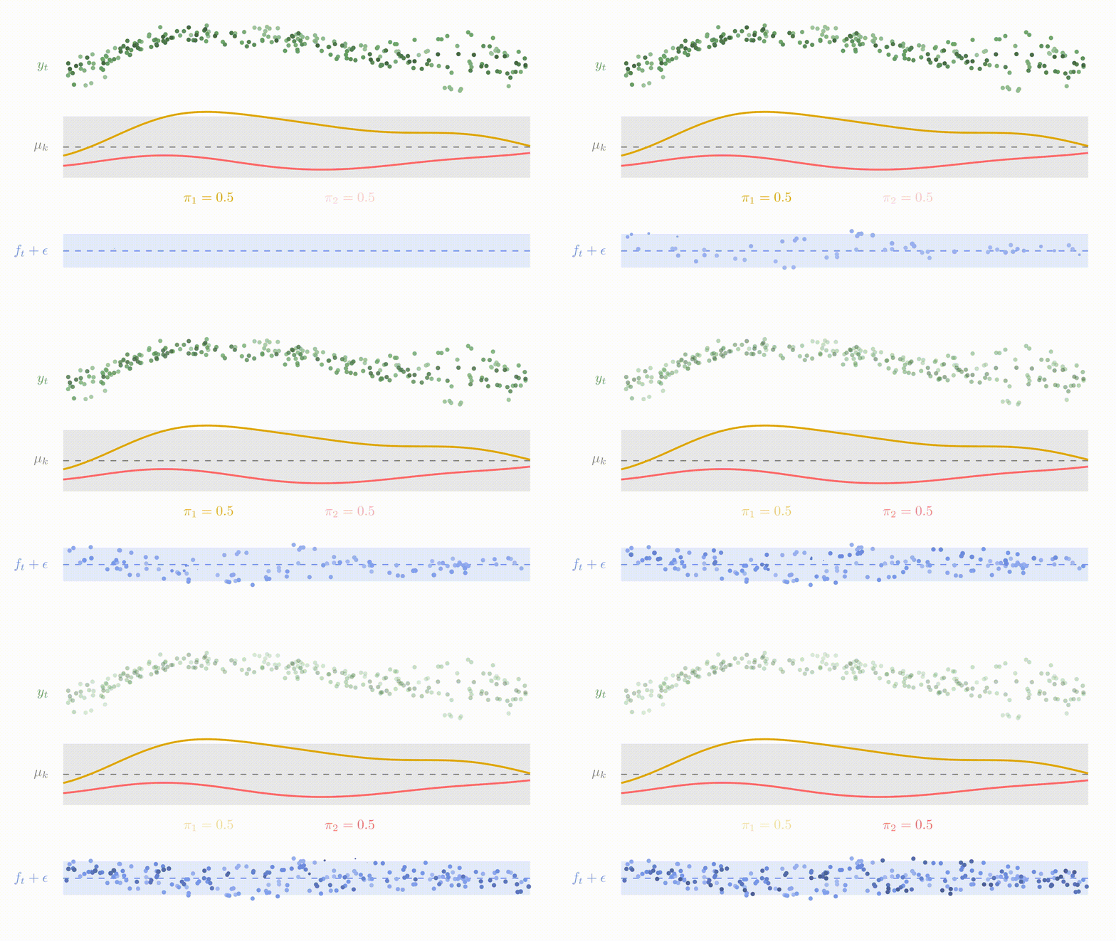
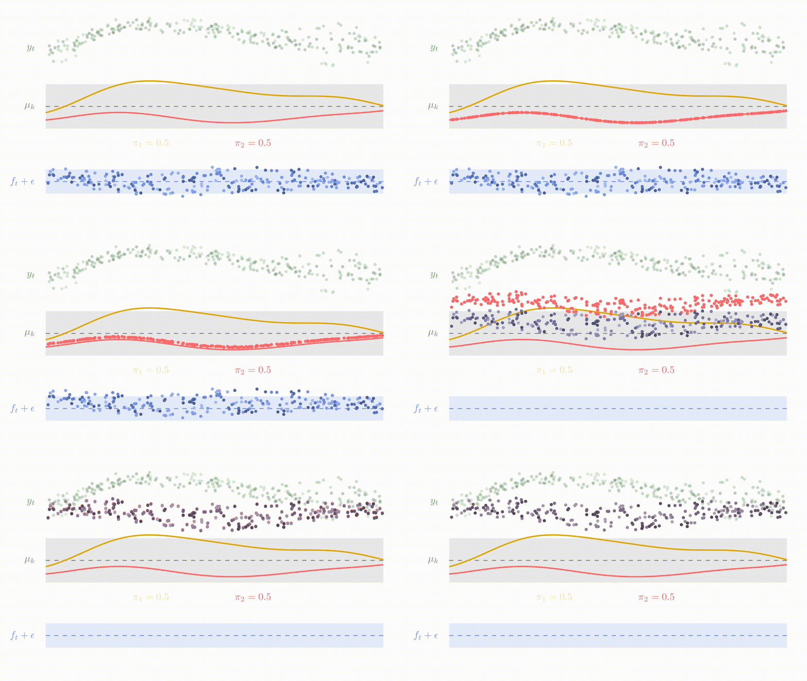
Adding some clustering into Multi-Task GPs

\(\rightarrow\) Mixture of multi-task GPs:

\[y_t = \mu_0 + f_t + \epsilon_t, \hspace{3cm} \forall t = 1, \dots, T\]

with:

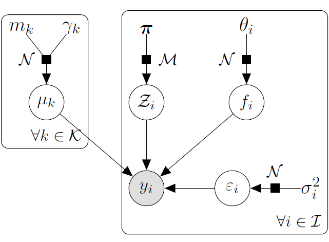
\(\color{green}{Z_{t}} \sim \mathcal{M}(1, \color{green}{\boldsymbol{\pi}}), \ \perp \!\!\! \perp_t,\)

\(\mu_0 \sim \mathcal{GP}(m_0, K_0),\)
\(f_t \sim \mathcal{GP}(0, \Sigma_{\theta_t}), \ \perp \!\!\! \perp_t,\)
\(\epsilon_t \sim \mathcal{GP}(0, \sigma_t^2), \ \perp \!\!\! \perp_t.\)

It follows that:

\[y_t \mid \mu_0 \sim \mathcal{GP}(\mu_0, \Psi_t), \ \perp \!\!\! \perp_t\]

Adding some clustering into Multi-Task GPs

A unique underlying mean process might be too restrictive.

\(\rightarrow\) Mixture of multi-task GPs:

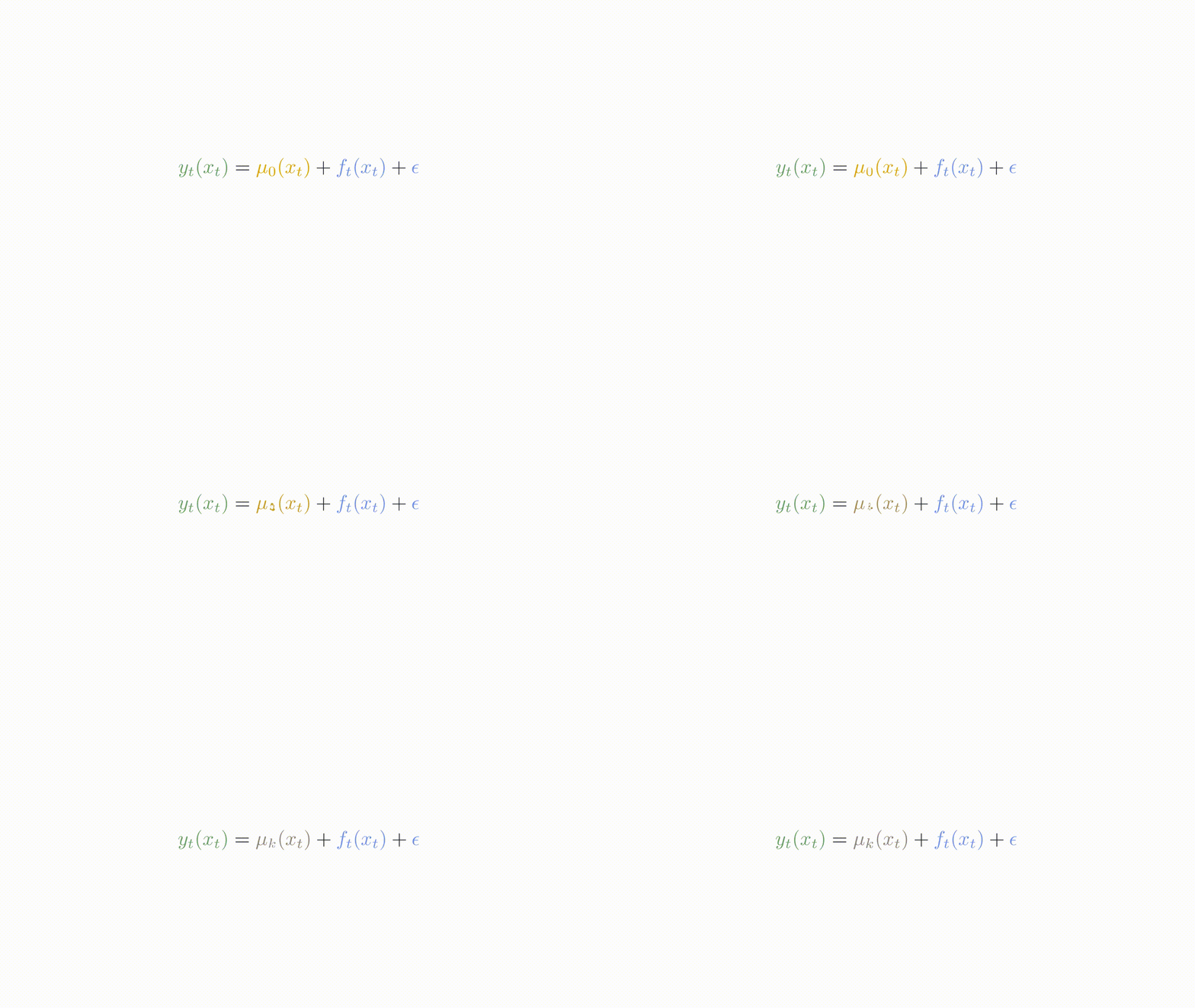
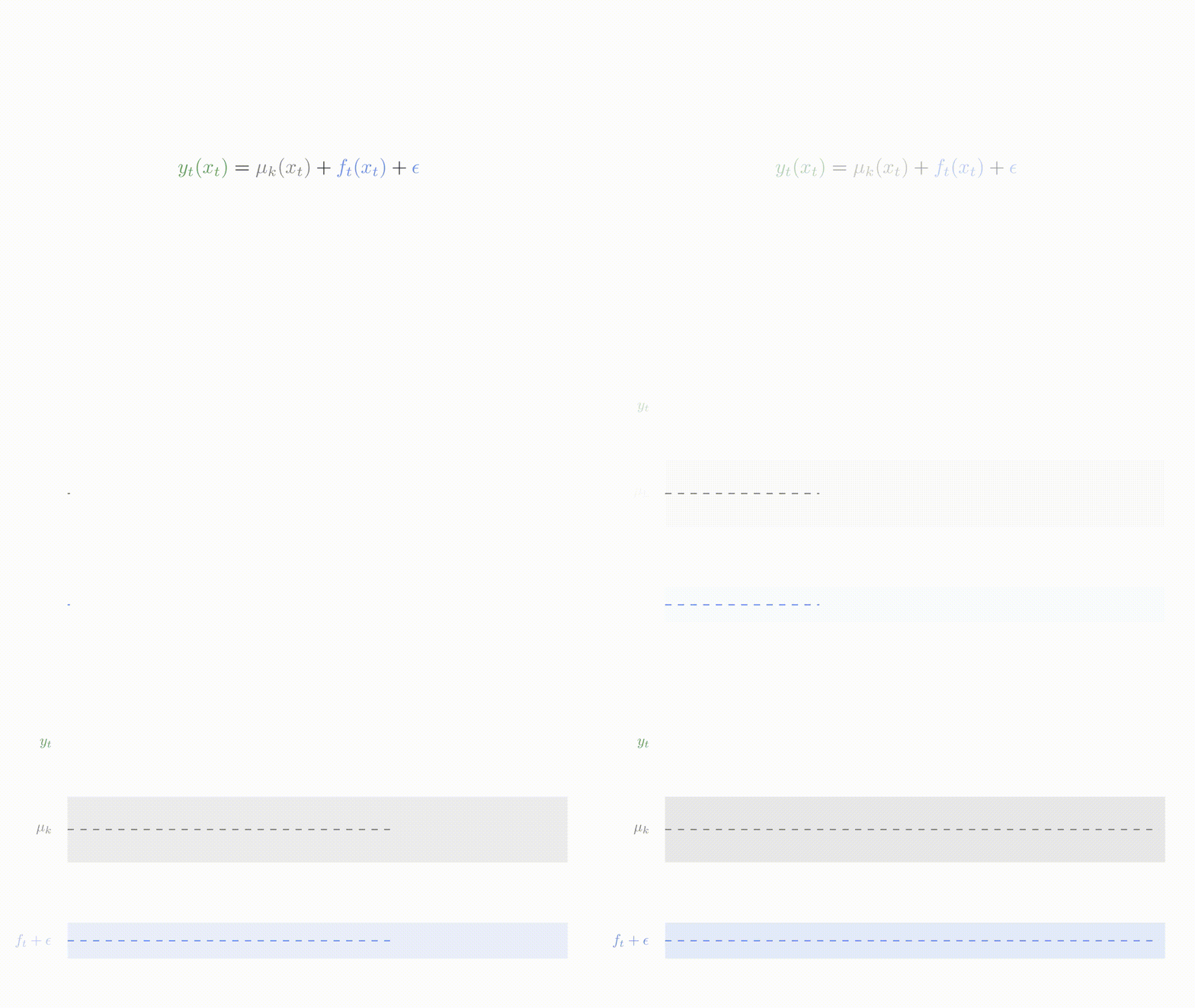
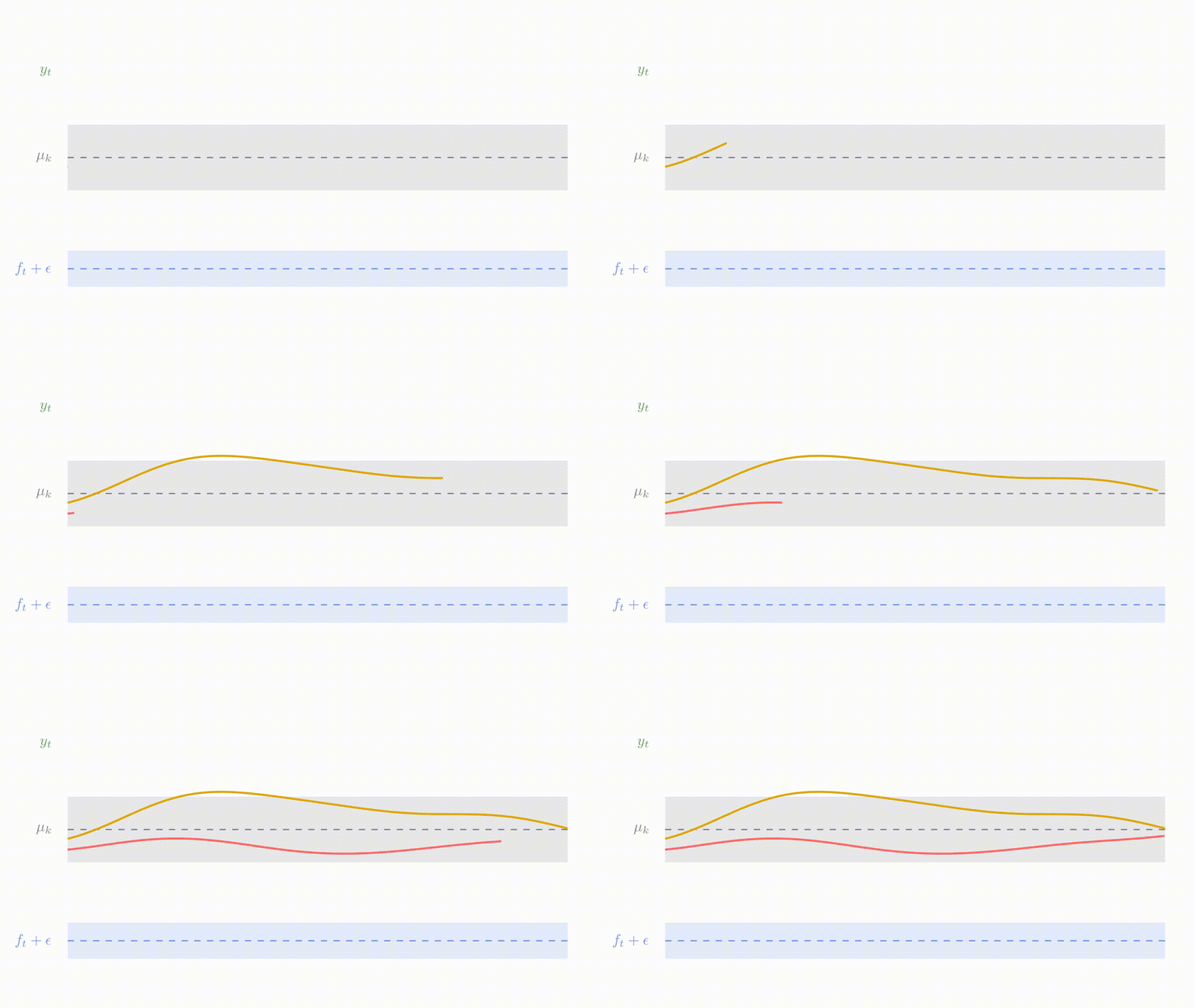
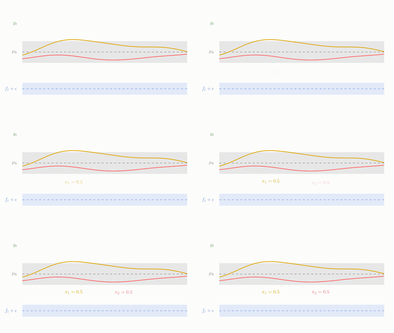
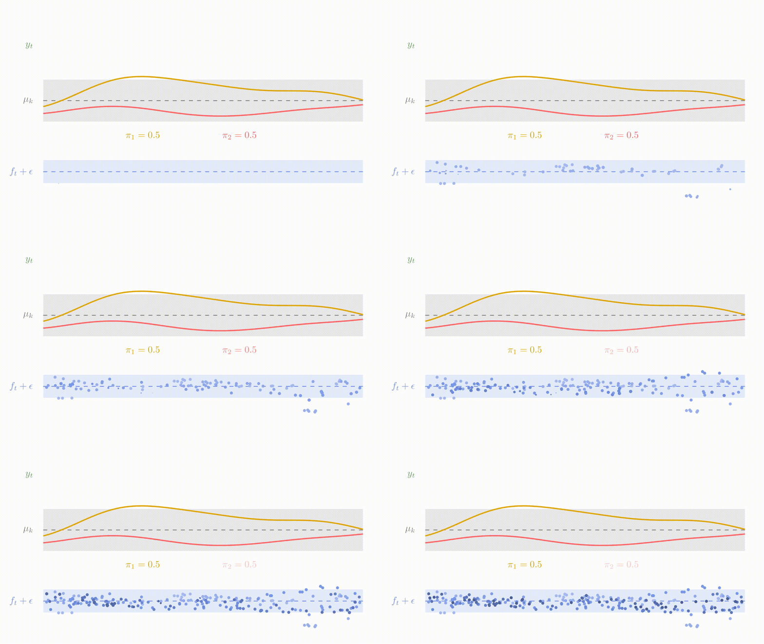
\[y_t \mid \{\color{green}{Z_{tk}} = 1 \} = \mu_{\color{green}{k}} + f_t + \epsilon_t, \hspace{3cm} \forall t = 1, \dots, T\]

with:

\(\color{green}{Z_{t}} \sim \mathcal{M}(1, \color{green}{\boldsymbol{\pi}}), \ \perp \!\!\! \perp_t,\)
\(\mu_{\color{green}{k}} \sim \mathcal{GP}(m_{\color{green}{k}}, \color{green}{C_{{k}}})\ \perp \!\!\! \perp_{\color{green}{k}},\)
\(f_t \sim \mathcal{GP}(0, \Sigma_{\theta_t}), \ \perp \!\!\! \perp_t,\)
\(\epsilon_t \sim \mathcal{GP}(0, \sigma_t^2), \ \perp \!\!\! \perp_t.\)

It follows that:

\[y_t \mid \mu_0 \sim \mathcal{GP}(\mu_0, \Psi_t), \ \perp \!\!\! \perp_t\]

Adding some clustering into Multi-Task GPs

A unique underlying mean process might be too restrictive.

\(\rightarrow\) Mixture of multi-task GPs:

\[y_t \mid \{\color{green}{Z_{ik}} = 1 \} = \mu_{\color{green}{k}} + f_t + \epsilon_t, \hspace{3cm} \forall t = 1, \dots, T\]

with:

\(\color{green}{Z_{t}} \sim \mathcal{M}(1, \color{green}{\boldsymbol{\pi}}), \ \perp \!\!\! \perp_t,\)
\(\mu_{\color{green}{k}} \sim \mathcal{GP}(m_{\color{green}{k}}, \color{green}{C_{{k}}})\ \perp \!\!\! \perp_{\color{green}{k}},\)
\(f_t \sim \mathcal{GP}(0, \Sigma_{\theta_t}), \ \perp \!\!\! \perp_t,\)
\(\epsilon_t \sim \mathcal{GP}(0, \sigma_t^2), \ \perp \!\!\! \perp_t.\)

It follows that:

\[y_t \mid \{ \boldsymbol{\mu} , \color{green}{\boldsymbol{\pi}} \} \sim \sum\limits_{k=1}^K{ \color{green}{\pi_k} \ \mathcal{GP}\Big(\mu_{\color{green}{k}}, \Psi_t^\color{green}{k} \Big)}, \ \perp \!\!\! \perp_t\]

Generative modelling assumptions

Variational EM

E step: \[ \begin{align} \hat{q}_{\boldsymbol{\mu}}(\boldsymbol{\mu}) &= \color{green}{\prod\limits_{k = 1}^K} \mathcal{N}(\mu_\color{green}{k};\hat{m}_\color{green}{k}, \hat{\textbf{C}}_\color{green}{k}) , \hspace{2cm} \hat{q}_{\boldsymbol{Z}}(\boldsymbol{Z}) = \prod\limits_{t = 1}^T \mathcal{M}(Z_t;1, \color{green}{\boldsymbol{\tau}_t}) \end{align} \] M step:

\[ \begin{align*} \hat{\Theta} &= \underset{\Theta}{\arg\max} \sum\limits_{k = 1}^{K}\sum\limits_{t = 1}^{T}\tau_{tk}\ \mathcal{N} \left( \mathbf{y}_t; \ \hat{m}_k, \boldsymbol{\Psi}_{\color{blue}{\theta_t}, \color{blue}{\sigma_t^2}} \right) - \dfrac{1}{2} \textrm{tr}\left( \mathbf{\hat{C}}_k\boldsymbol{\Psi}_{\color{blue}{\theta_t}, \color{blue}{\sigma_t^2}}^{-1}\right) \\ & \hspace{1cm} + \sum\limits_{k = 1}^{K}\sum\limits_{t = 1}^{T}\tau_{tk}\log \color{green}{\pi_{k}} \end{align*} \]

Cluster-specific and mixture predictions

Multi-Task posterior for each cluster:

\[ p(y_*(\mathbf{x}^{p}) \mid \color{green}{Z_{*k}} = 1, y_*(\mathbf{x}_{*}), \textbf{y}) = \mathcal{N} \Big( y_*(\mathbf{x}^{p}); \ \hat{\mu}_{*}^\color{green}{k}(\mathbf{x}^{p}) , \hat{\Gamma}_{pp}^\color{green}{k} \Big), \forall \color{green}{k}, \]

\(\hat{\mu}_{*}^\color{green}{k}(\mathbf{x}^{p}) = \hat{m}_\color{green}{k}(\mathbf{x}^{p}) + \Gamma^\color{green}{k}_{p*} {\Gamma^\color{green}{k}_{**}}^{-1} (y_*(\mathbf{x}_{*}) - \hat{m}_\color{green}{k} (\mathbf{x}_{*}))\)
\(\hat{\Gamma}_{pp}^\color{green}{k} = \Gamma_{pp}^\color{green}{k} - \Gamma_{p*}^\color{green}{k} {\Gamma^{\color{green}{k}}_{**}}^{-1} \Gamma^{\color{green}{k}}_{*p}\)

Predictive multi-task GPs mixture:

\[p(y_*(\textbf{x}^p) \mid y_*(\textbf{x}_*), \textbf{y}) = \color{green}{\sum\limits_{k = 1}^{K} \tau_{*k}} \ \mathcal{N} \big( y_*(\mathbf{x}^{p}); \ \hat{\mu}_{*}^\color{green}{k}(\textbf{x}^p) , \hat{\Gamma}_{pp}^\color{green}{k}(\textbf{x}^p) \big).\]

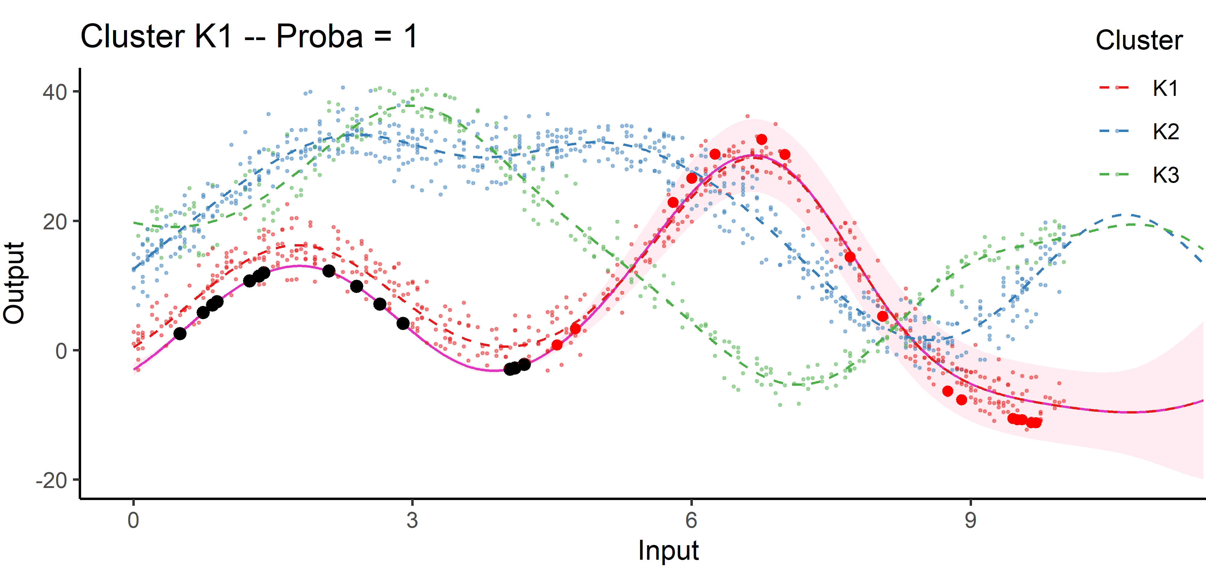
An image is still worth many words

A unique mean process can struggle to capture relevant signals in presence of group structures.

An image is still worth many words

By identifying the underlying clustering structure, we can discard unnecessary information and provide enhanced predictions as well as lower uncertainty.

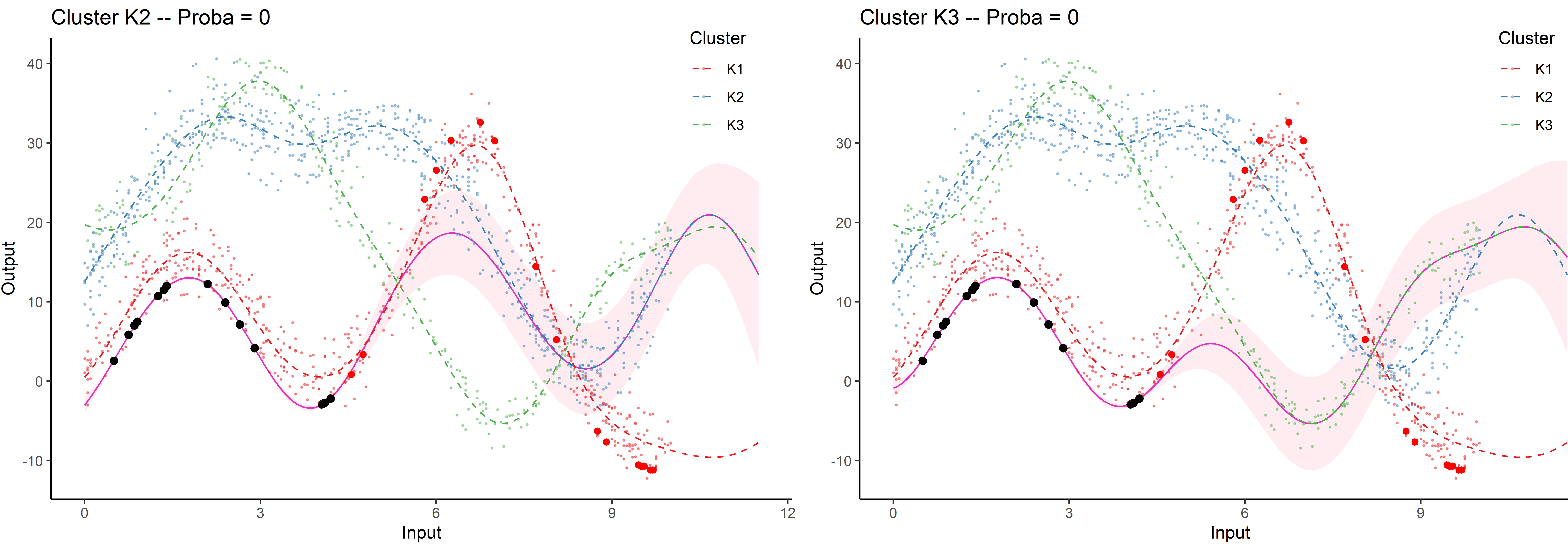
Saved by the weights

Each cluster-specific prediction is weighted by its membership probability \(\color{green}{\tau_{*k}}\).

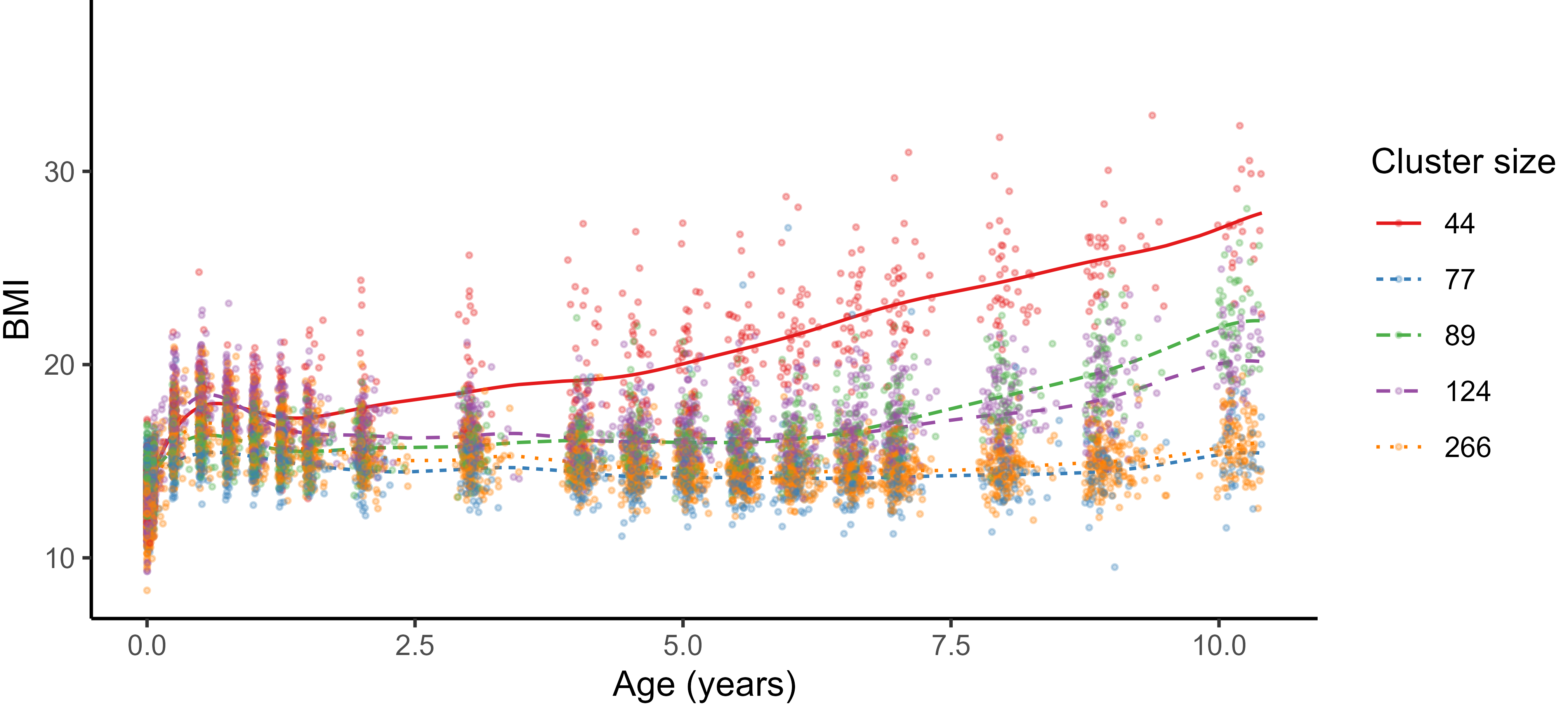
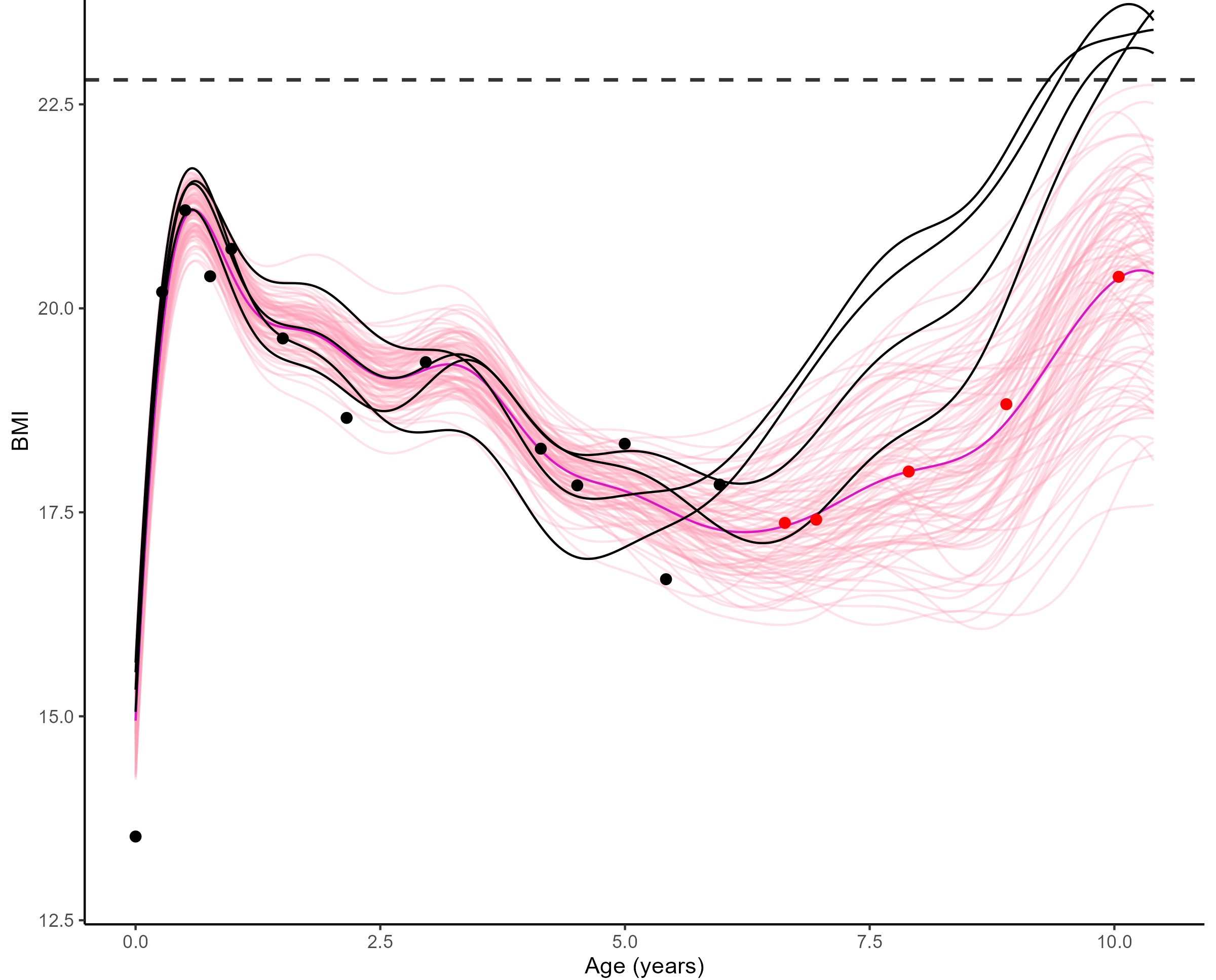
Practical application: follow up of BMI during childhood

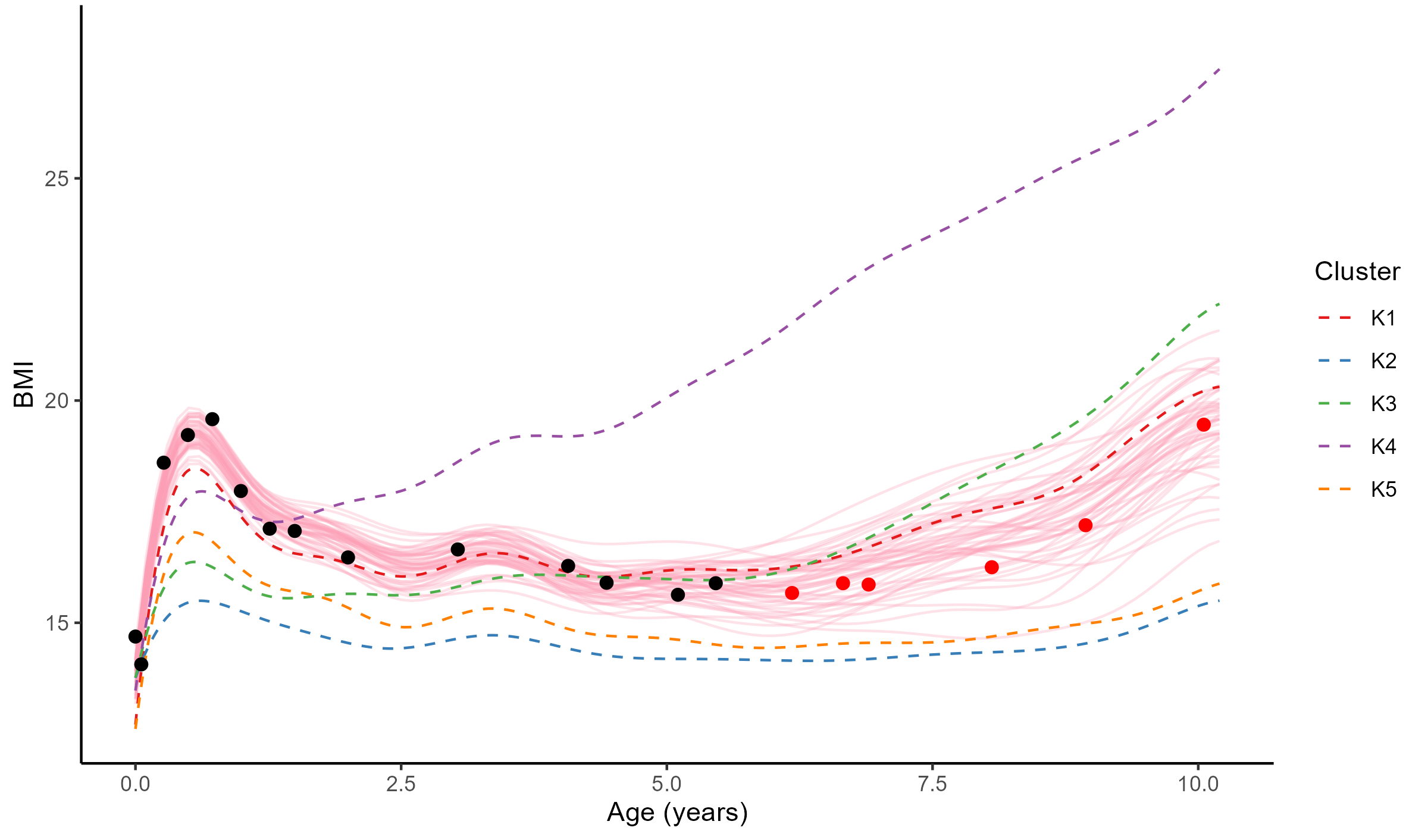
Forecasting long term evolution of BMI

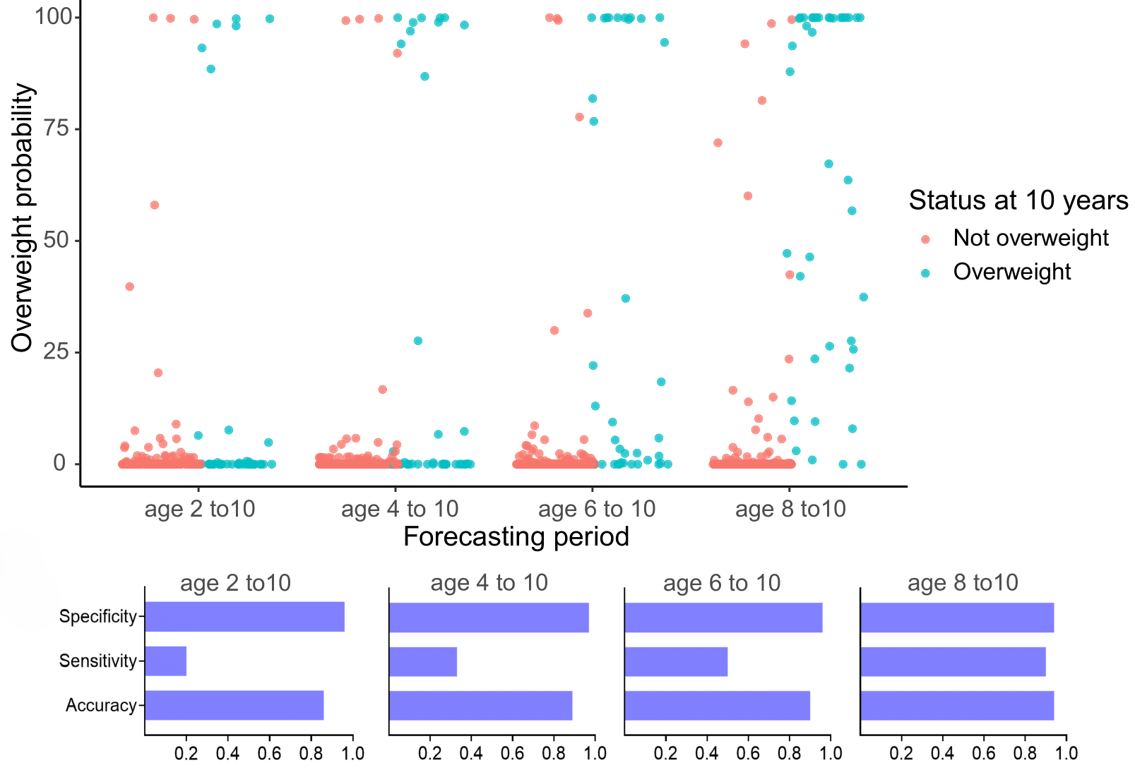
Leveraging the uncertainty quantification of GPs

Deriving downstream tools for practitioners

Uncertainty quantification provides valuable information to practitioners to make decisions based on probabilistic statements, like the risk of overweight at 10 years.

Two sides of the same coin?

Multi-Output GPs

flexible,
expressive,
computationally expensive,
fragile inference,
ideal to capture correlations across different variables of interest,

Multi-Task GPs

parsimonious,
robust,
linear scaling,
no cross-correlations,
ideal to capture different realisations of the same phenomenon.

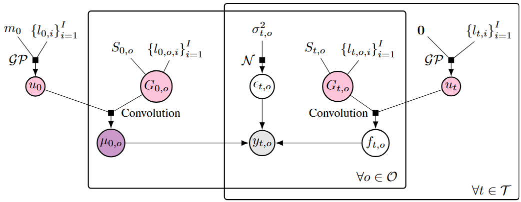
Generative model of MOMT GPs

\[\begin{bmatrix} y_t^{1} \\ \vdots \\ y_t^{O} \\ \end{bmatrix} = \begin{bmatrix} \mu_0 \\ \vdots \\ \mu_0 \\ \end{bmatrix} + \begin{bmatrix} f_t^{1} \\ \vdots \\ f_t^{O} \\ \end{bmatrix} + \begin{bmatrix} \epsilon_t^{1} \\ \vdots \\ \epsilon_t^{O} \\ \end{bmatrix}, \hspace{3cm} \forall t = 1, \dots, T\]

\(\mu_0 \sim \mathcal{GP}(m_0, K_0),\)
\(\begin{bmatrix} f_t^{1} \\ \vdots \\ f_t^{O} \\ \end{bmatrix} \sim \mathcal{GP}(0, \Sigma_{\theta_t}), \ \perp \!\!\! \perp_t,\)
\(\begin{bmatrix} \epsilon_t^{1} \\ \vdots \\ \epsilon_t^{O} \\ \end{bmatrix} \sim \mathcal{GP}(0, \begin{bmatrix} {\sigma_t^{1}}^O \\ \vdots \\ {\sigma_{t}^O}^2 \\ \end{bmatrix} \times I_O), \ \perp \!\!\! \perp_t.\)

All mathematical objects from Multi-Task GPs are now extended with stacked Outputs.

Compatible assumptions, different mechanisms

MT GPs share information through the mean, and make no assumptions on the covariance.
MO GPs share information through the covariance, and make no assumptions on the mean.

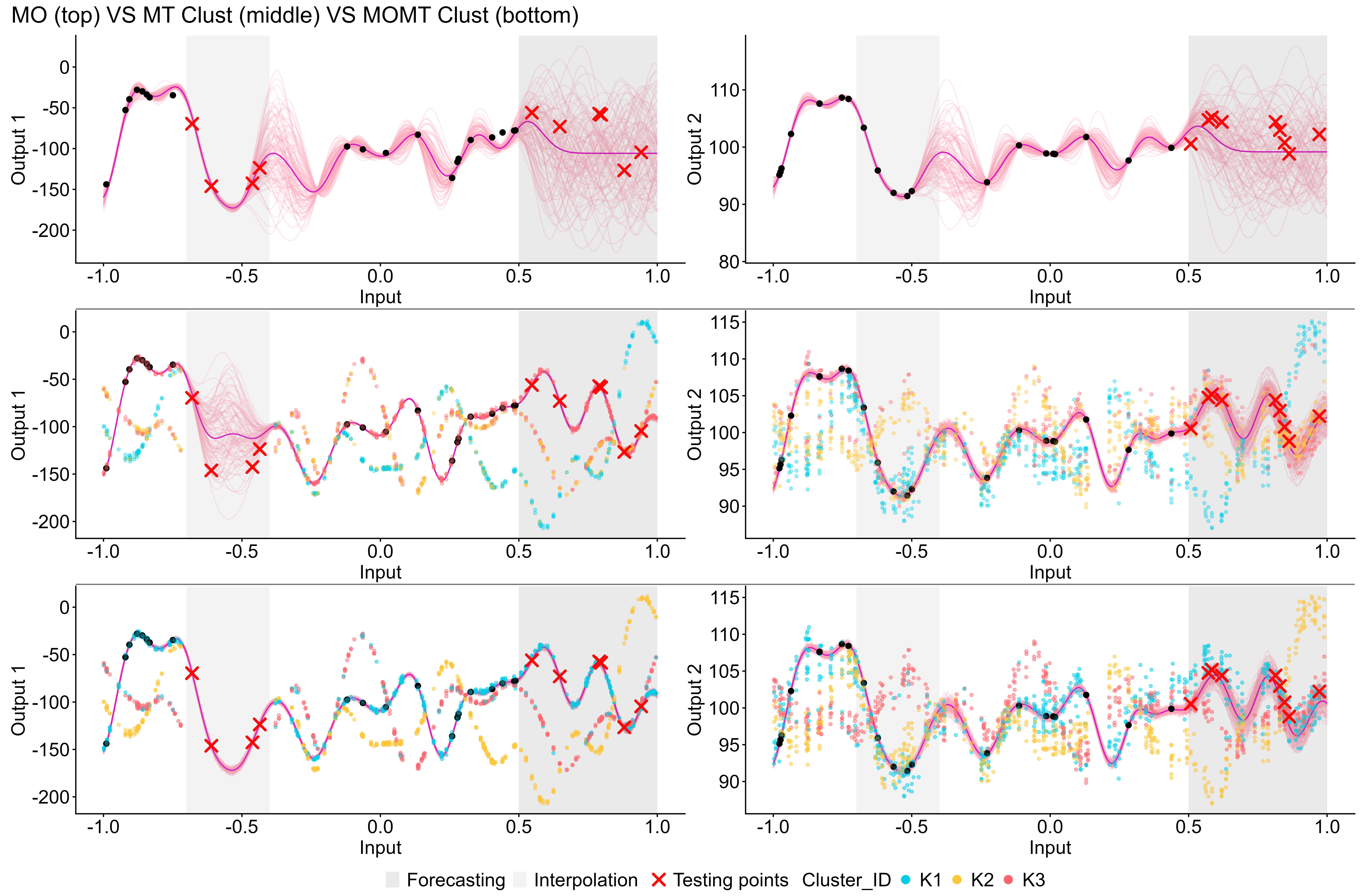
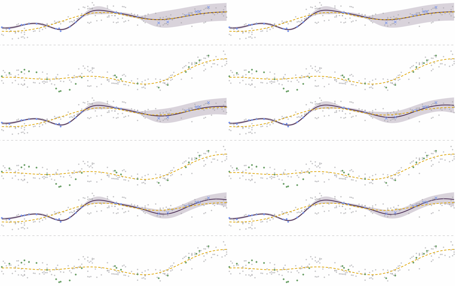
Do we really get the best of both worlds?

Swimming performances prediction with MOMT

Feel free to test it on your data

Historical R package MagmaClustR for multi-task GPs.

Brand new Jax-based library that comes with:

considerable speed-ups (JIT, GPU computations),
a native API designed around MO/MT/MOMT concepts,
Kernax, an efficient and modular Jax library for kernels,

This afternoon you can follow the dedicated tutorials.

Let’s rewind the whole story

Let’s rewind the whole story

Let’s rewind the whole story

Take home messages

Multi-Ouput / Multi-Task: the same mathematical problem can hide different intuitions on the data and lead to dedicated modelling paradigms,
Both Inputs and Outputs can be multidimensional (i.e. have multiple Channels),
Both the mean and covariance parameters can be leveraged to share information,
Modelling jointly data coming from several sources can costs roughly the same as independent modelling, but can improve dramatically predictive capacities.

Rule of thumb:

Output nature	Framework	Complexity
Independant variables of interest	Single-Task	\(\color{red}{O}\times\mathcal{O}(N^3)\)
Correlated variables of interest	Multi-Output	\(\mathcal{O}(\color{red}{O}^3 N^3)\)
Occurences of the same phenomenon	Multi-Task	\(\mathcal{O}(\color{blue}{T} \times N^3)\)
Occurences of correlated variables	Multi-Task-Multi-Output	\(\mathcal{O}(\color{blue}{T}\times\color{red}{O}^3 N^3)\)

The crew expanding all this

We are currently working on some nice extensions with a great team of PhD students!

Alexia Grenouillat - Simon Lejoly - Térence Viellard

Some problems we are currently tackling (at least trying to):

Develop a new MO strategy to combine modular GPs through tailored architectures,
Integrate useful extensions (sparse approx, non-Gaussian likelihood, …) within MIMOSA,
Scalability in the number of inputs, outputs, tasks, input dimensions,
Hopefully many other problems that we’ll be happy to discuss with you!

Thank you for your attention!

Multi-Output and Multi-Task Gaussian Processes

Arthur Leroy - GABI & MIA Paris Saclay, INRAE

Gaussian Process Summer School - 15/09/2026

It all starts with observations from multiple sources …

It all starts with observations from multiple sources …

… but sometimes we are not measuring the same things …

Let’s play a game

So. We restart with observations from multiple sources …

… but sometimes we are not measuring the same things …

… sometimes data come in successive batches …

… sometimes data come in successive batches …

… sometimes data come in successive batches …

… sometimes data come in successive batches …

… many things can be multidimensional …

… I feel like we are spiraling …

… among many other difficulties …

… among many other difficulties …

… or all of them at once.

Multi-Task? Multi-Output? A proposed formalisation

Gaussian process: a prior distribution over functions

Gaussian process: all you need is a posterior

Have you had enough introductions to GPs?

Another one for the road

A quick one I promise

See, already done. Let the real fun begin!

Forecasting with a unique GP

Forecasting with a unique GP

A long history of old and modern Multi-Output strategies

Multi-Output GPs: exploiting explicit correlations

Intuition behind the Kronecker formulation

Multi-Output GPs: the ideal case

Intrinsic Corregionalisation Model (ICM)

Linear Model of Corregionalisation (LMC)

Process Convolution (PC)

Generative flexibility

Generative flexibility

Some limits of Multi-Output GPs

Another paradigm: Multi-Task GPs with shared mean process

Generative modelling assumptions

Generative modelling assumptions

Generative modelling assumptions

Generative modelling assumptions

Generative modelling assumptions

Generative modelling assumptions

Generative modelling assumptions

Generative modelling assumptions

Generative modelling assumptions

EM algorithm

Covariance structure assumption and computational complexity

Prediction

Prediction: the key idea

Final prediction: the good old GP formula

A GIF is worth a thousand words

A GIF is worth a thousand words

Comparison with single GP regression

What happens with multi-dimensional inputs?

Yet another comparison with single GP regression

Some limits of Multi-Task GPs

Adding some clustering into Multi-Task GPs

Adding some clustering into Multi-Task GPs

Adding some clustering into Multi-Task GPs

Generative modelling assumptions

Generative modelling assumptions

Generative modelling assumptions

Generative modelling assumptions

Generative modelling assumptions

Generative modelling assumptions

Generative modelling assumptions

Generative modelling assumptions

Variational EM

Cluster-specific and mixture predictions

An image is still worth many words

An image is still worth many words

Saved by the weights

Practical application: follow up of BMI during childhood

Forecasting long term evolution of BMI

Leveraging the uncertainty quantification of GPs

Deriving downstream tools for practitioners

Two sides of the same coin?

Generative model of MOMT GPs

Multi-Output and Multi-Task
Gaussian Processes