---

Multi-Output and Multi-Task
Gaussian Processes

---

Arthur Leroy - GABI & MIA Paris Saclay, INRAE

Séminaire GiBBS - 19/01/2026

It all starts with observations from multiple sources …

It all starts with observations from multiple sources …

… where the input space can be multidimensional as well …

… but sometimes we are not measuring the same things …

… among many other difficulties …

• Irregular time series (in number of observations and location),
• A few observations for each source,

… among many other difficulties …

• Irregular input measurements (in number of observations and location),
• A few observations for each source,
• Many different sources.

… or all of them at once.

Supervised learning: the general framework

\[y = \color{orange}{f}(x) + \epsilon\]

where:

• \(x\) is the input variable (typically time, location, any continuum),
• \(y\) is the output variable (any measurement of interest),
• \(\epsilon\) is the noise, a random error term,
• \(\color{orange}{f}\) is a random function encoding the relationship between input and output data.

All supervised learning problems require to retrieve the most reliable function \(\color{orange}{f}\), using observed data \(\{(x_1, y_1), \dots, (x_n, y_n) \}\), to perform predictions when observing new input data \(x_{n+1}\).

Gaussian process: a prior distribution over functions

\[y = \color{orange}{f}(x) + \epsilon\]

No restrictions on \(\color{orange}{f}\) but a prior distribution on a functional space: \(\color{orange}{f} \sim \mathcal{GP}(m(\cdot),C(\cdot,\cdot))\)

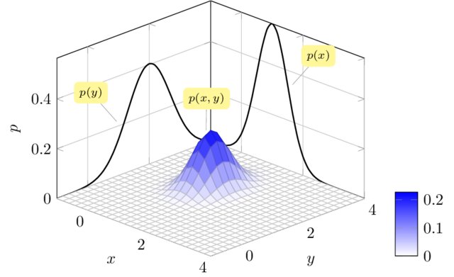
We can think of a Gaussian process as the extension to infinity of multivariate Gaussians:
      \(x \sim \mathcal{N}(m , \sigma^2)\) in \(\mathbb{R}\),       \(\begin{pmatrix} x_1 \\ x_2 \\ \end{pmatrix} \sim \mathcal{N} \left( \ \begin{pmatrix} m_1 \\ m_2 \\ \end{pmatrix}, \begin{bmatrix} C_{1,1} & C_{1,2} \\ C_{2,1} & C_{2,2} \end{bmatrix} \right)\) in \(\mathbb{R}^2\)

     
Credits: Raghavendra Selvan

Gaussian process: a prior distribution over functions

\[y = \color{orange}{f}(x) + \epsilon\]

No restrictions on \(\color{orange}{f}\) but a prior distribution on a functional space: \(\color{orange}{f} \sim \mathcal{GP}(m(\cdot),C(\cdot,\cdot))\)

We can think of a Gaussian process as the extension to infinity of multivariate Gaussians:

\[p(f_1, f_2, \ldots, f_N, \ldots \mid \mathbf{x}) = \mathcal{N}\left( \begin{bmatrix} m(x_1) \\ m(x_2) \\ \vdots \\ m(x_N) \\ \vdots \end{bmatrix}, \begin{bmatrix} C(x_1,x_1) & C(x_1,x_2) & \cdots & C(x_1,x_N) & \cdots \\ C(x_2,x_1) & C(x_2,x_2) & \cdots & C(x_2,x_N) & \cdots \\ \vdots & \vdots & \ddots & \vdots & \\ C(x_N,x_1) & C(x_N,x_2) & \cdots & C(x_N,x_N) & \cdots \\ \vdots & \vdots & & \vdots & \ddots \end{bmatrix} \right)\]

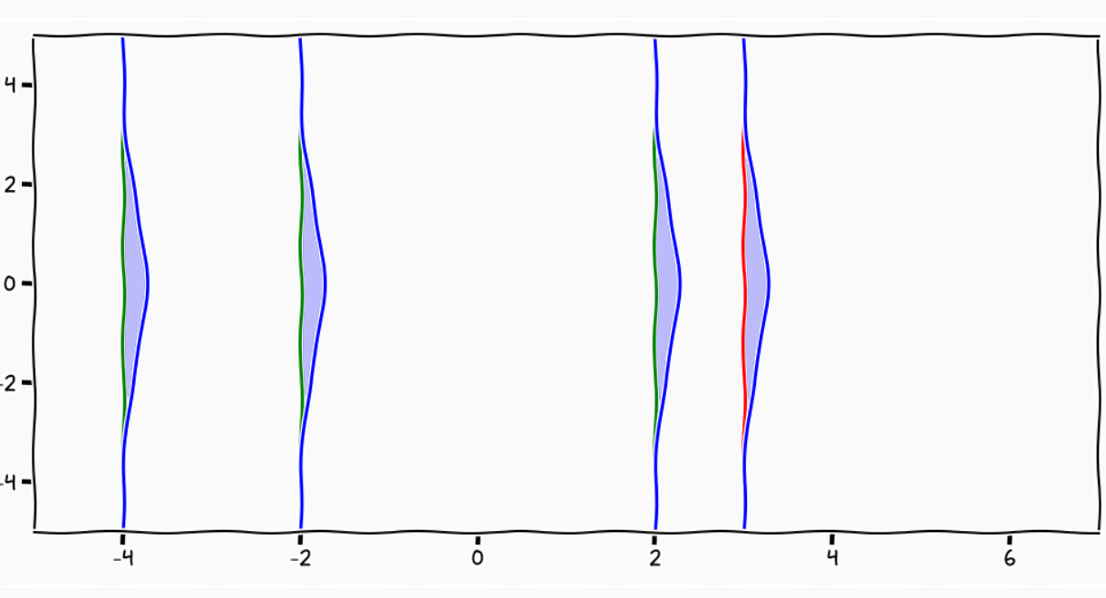
A GP is like a long cake and each slice is a Gaussian

Credits: Carl Henrik Ek

A GP is like an infinitely long cake and each slice is a Gaussian

Credits: Carl Henrik Ek

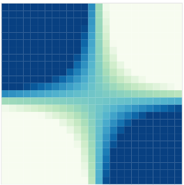
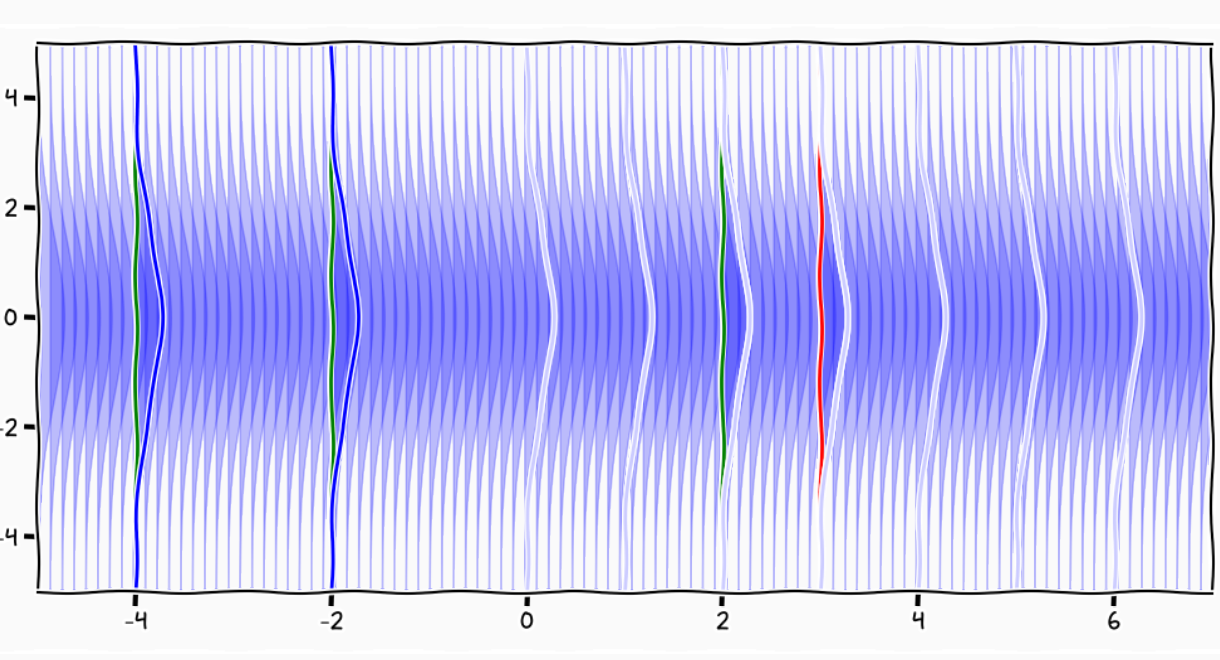
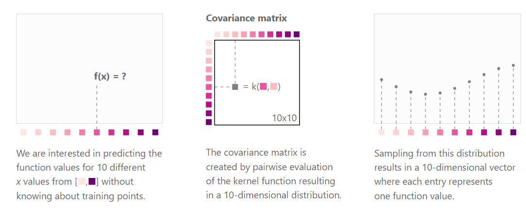
Kernels and covariance functions

Kernels (or covariance functions) \(C(\cdot, \cdot)\) define the covariance structure of functions sampled from a GP. Formally, we fill the covariance matrix \(K\) such that:

\[cov(f(x), f(x^{\prime})) = C(x, x^{\prime}) = \left[C \right]_{x, x^{\prime}}.\]

https://distill.pub/2019/visual-exploration-gaussian-processes/

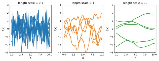
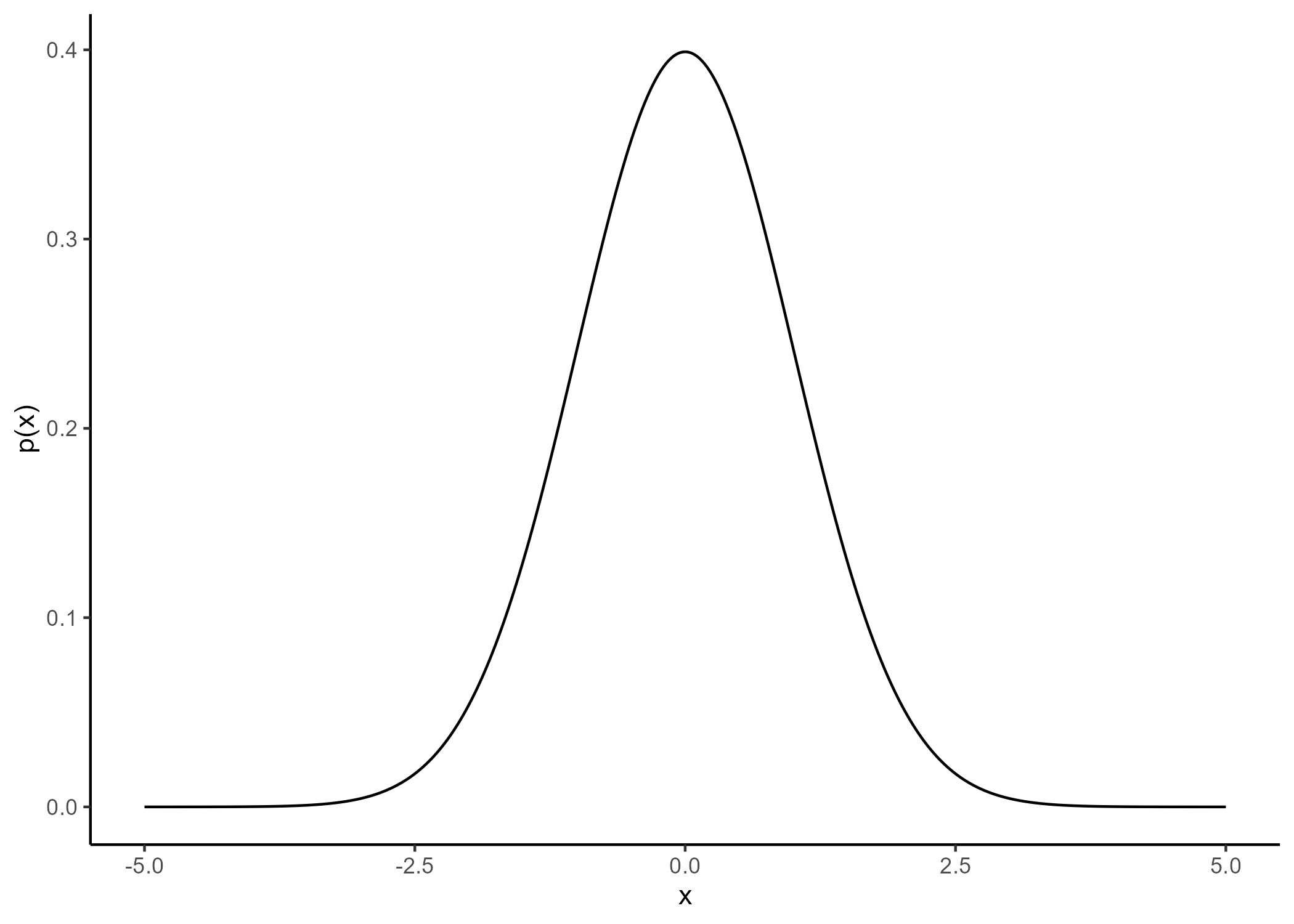
Covariance functions: Squared Exponential kernel

While \(m(\cdot)\) is often assumed to be \(0\), the covariance structure is critical and defined through tailored kernels. For instance, the Squared Exponential (or RBF) kernel is expressed as: \[C_{SE}(x, x^{\prime}) = s^2 \exp \Bigg(-\dfrac{(x - x^{\prime})^2}{2 \ell^2}\Bigg)\]

     

Covariance functions: Periodic kernel

To model phenomenon exhibiting repeting patterns, one can leverage the Periodic kernel: \[C_{perio}(x, x^{\prime}) = s^2 \exp \Bigg(- \dfrac{ 2 \sin^2 \Big(\pi \frac{\mid x - x^{\prime}\mid}{p} \Big)}{\ell^2}\Bigg)\]

     

Covariance functions: Linear kernel

We can even consider linear regression as a particular GP problem, by using the Linear kernel: \[C_{lin}(x, x^{\prime}) = s_a^2 + s_b^2 (x - c)(x^{\prime} - c )\]

     

We can learn optimal values of hyper-parameters from data through maximum likelihood.

Gaussian process regression model

Given observed data \(\mathbf{y} = (y_1, \dots, y_n)^T\) at inputs \(\mathbf{x} = (x_1, \dots, x_n)^T\), we assume:

\[y_i = \color{orange}{f}(x_i) + \epsilon_i, \hspace{1cm} \forall i = 1, \dots, n\]

with

• \(\color{orange}{f} \sim \mathcal{GP}(m(\cdot), C_{\theta}(\cdot, \cdot))\),
• \(\epsilon_i \sim \mathcal{N}(0, \sigma^2)\), independent noise terms.

The vector of observations \(\mathbf{y}\) follows a multivariate Gaussian distribution:

\[\mathbf{y} \sim \mathcal{N}(m(\mathbf{x}), C_{\theta}(\mathbf{x}, \mathbf{x}) + \sigma^2 I)\]

where \(C_{\theta}(\mathbf{x}, \mathbf{x})\) is the covariance matrix evaluated at inputs \(\mathbf{x}\), with hyper-parameters \(\theta\).

Optimising hyper-parameters of the kernel

The log-marginal likelihood of observed data \(\mathbf{y}\) given inputs \(\mathbf{x}\) and hyper-parameters \(\theta\) is: \[\log p(\mathbf{y} \mid \mathbf{x}, \theta) = -\frac{1}{2} \mathbf{y}^T (C_{\theta} + \sigma^2 I )^{-1} \mathbf{y} - \frac{1}{2} \log |C_{\theta} + \sigma^2 I| - \frac{n}{2} \log 2\pi.\]

We can optimise hyper-parameters \(\theta\) by maximizing the log-marginal likelihood using gradient-based methods.

Source: 10.48550/arXiv.2511.12550

Gaussian process: all you need is a posterior

The Gaussian property induces that unobserved points have no influence on inference:

\[ \int \underbrace{p(f_{\color{grey}{obs}}, f_{\color{purple}{mis}})}_{\mathcal{GP}(m, C)} \ \mathrm{d}f_{\color{purple}{mis}} = \underbrace{p(f_{\color{grey}{obs}})}_{\mathcal{N}(m_{\color{grey}{obs}}, C_{\color{grey}{obs}})} \]

This crucial trick allows us to learn function properties from finite sets of observations. More generally, Gaussian processes are closed under conditioning and marginalisation.

\[ \begin{bmatrix} f_{\color{grey}{o}} \\ f_{\color{purple}{m}} \\ \end{bmatrix} \sim \mathcal{N} \left( \begin{bmatrix} m_{\color{grey}{o}} \\ m_{\color{purple}{m}} \\ \end{bmatrix}, \begin{pmatrix} C_{\color{grey}{o, o}} & C_{\color{grey}{o}, \color{purple}{m}} \\ C_{\color{purple}{m}, \color{grey}{o}} & C_{\color{purple}{m, m}} \end{pmatrix} \right)\]

While marginalisation serves for training, conditioning leads the key GP prediction formula:

\[f_{\color{purple}{m}} \mid f_{\color{grey}{o}} \sim \mathcal{N} \Big( m_{\color{purple}{m}} + C_{\color{purple}{m}, \color{grey}{o}} C_{\color{grey}{o, o}}^{-1} (f_{\color{grey}{o}} - m_{\color{grey}{o}}), \ \ C_{\color{purple}{m, m}} - C_{\color{purple}{m}, \color{grey}{o}} C_{\color{grey}{o, o}}^{-1} C_{\color{grey}{o}, \color{purple}{m}} \Big)\]

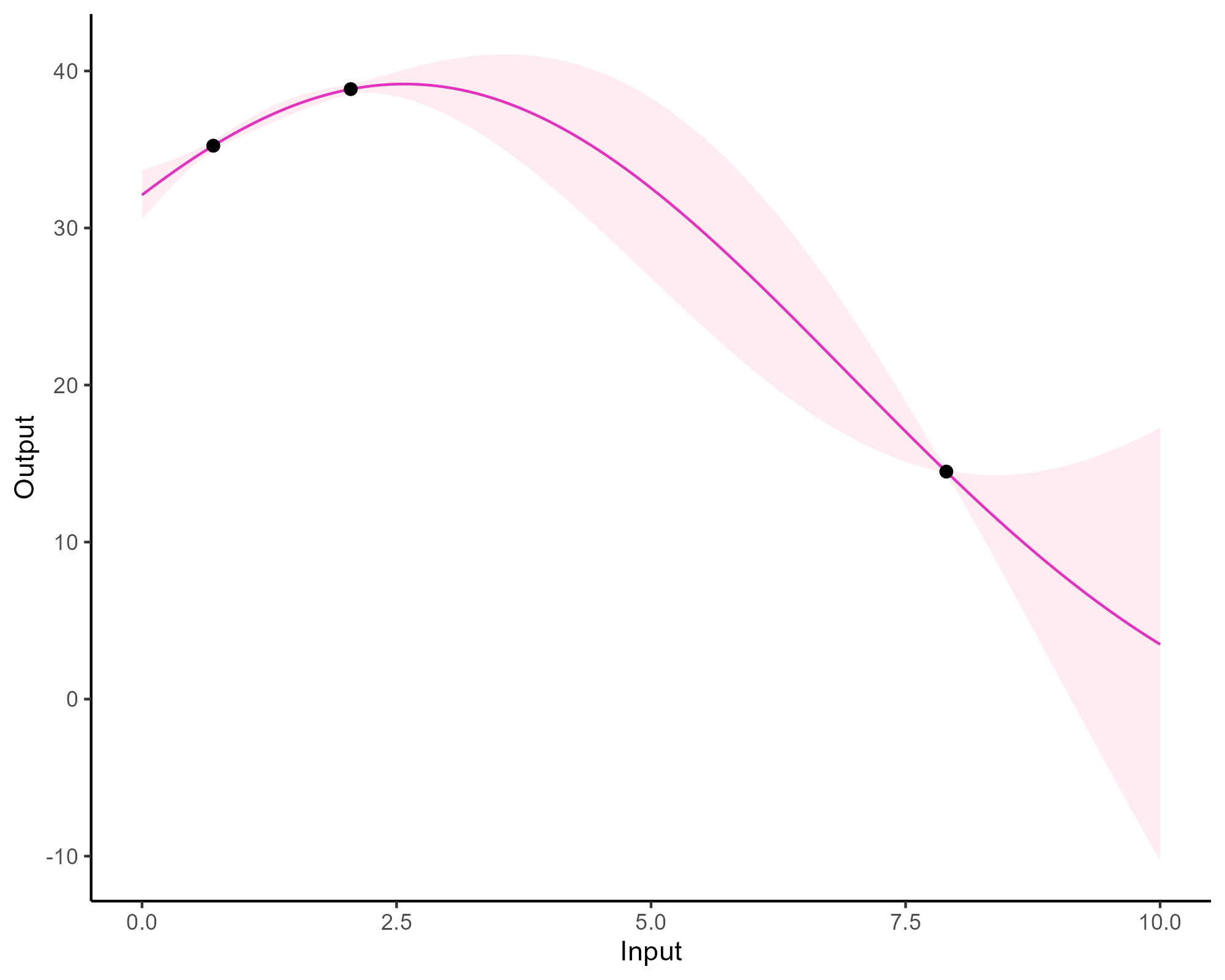
A visual summary of GP regression: prior and optimisation

\(f \sim \mathcal{GP}(0, C_{SE}(\cdot, \cdot))\)                 \(\hat{\theta} = \text{argmax}_{\theta} \log p(\mathbf{y} \mid \mathbf{x}, \theta)\)

Prediction: updating our knowledge about functions

\(f_{\color{purple}{m}} \mid f_{\color{grey}{o}} \sim \mathcal{N} \Big( m_{\color{purple}{m}} + C_{\color{purple}{m}, \color{grey}{o}} C_{\color{grey}{o, o}}^{-1} (f_{\color{grey}{o}} - m_{\color{grey}{o}}), \ \ C_{\color{purple}{m, m}} - C_{\color{purple}{m}, \color{grey}{o}} C_{\color{grey}{o, o}}^{-1} C_{\color{grey}{o}, \color{purple}{m}} \Big)\)

Prediction: updating our knowledge about functions

\(f_{\color{purple}{m}} \mid f_{\color{grey}{o}} \sim \mathcal{N} \Big( m_{\color{purple}{m}} + C_{\color{purple}{m}, \color{grey}{o}} C_{\color{grey}{o, o}}^{-1} (f_{\color{grey}{o}} - m_{\color{grey}{o}}), \ \ C_{\color{purple}{m, m}} - C_{\color{purple}{m}, \color{grey}{o}} C_{\color{grey}{o, o}}^{-1} C_{\color{grey}{o}, \color{purple}{m}} \Big)\)

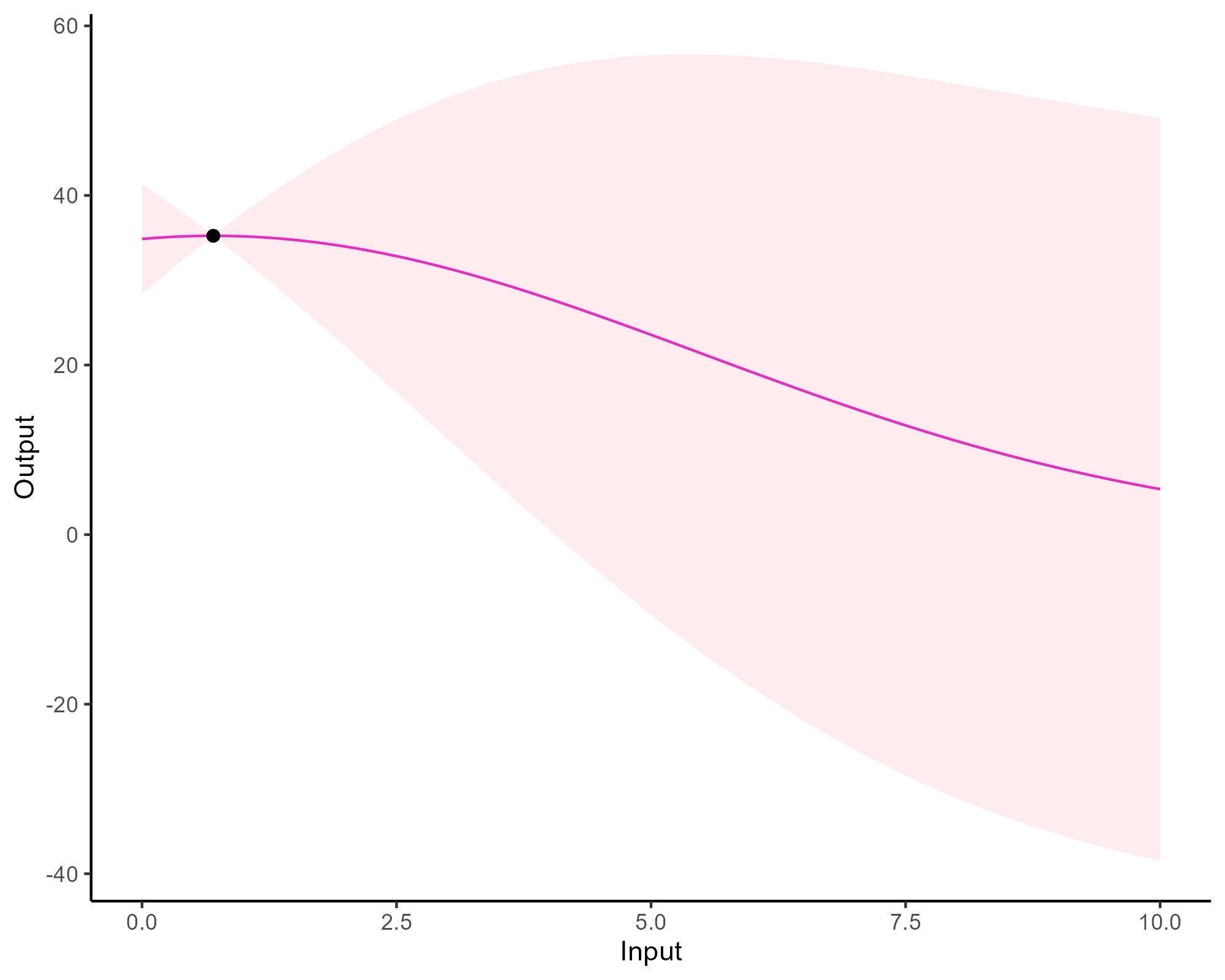
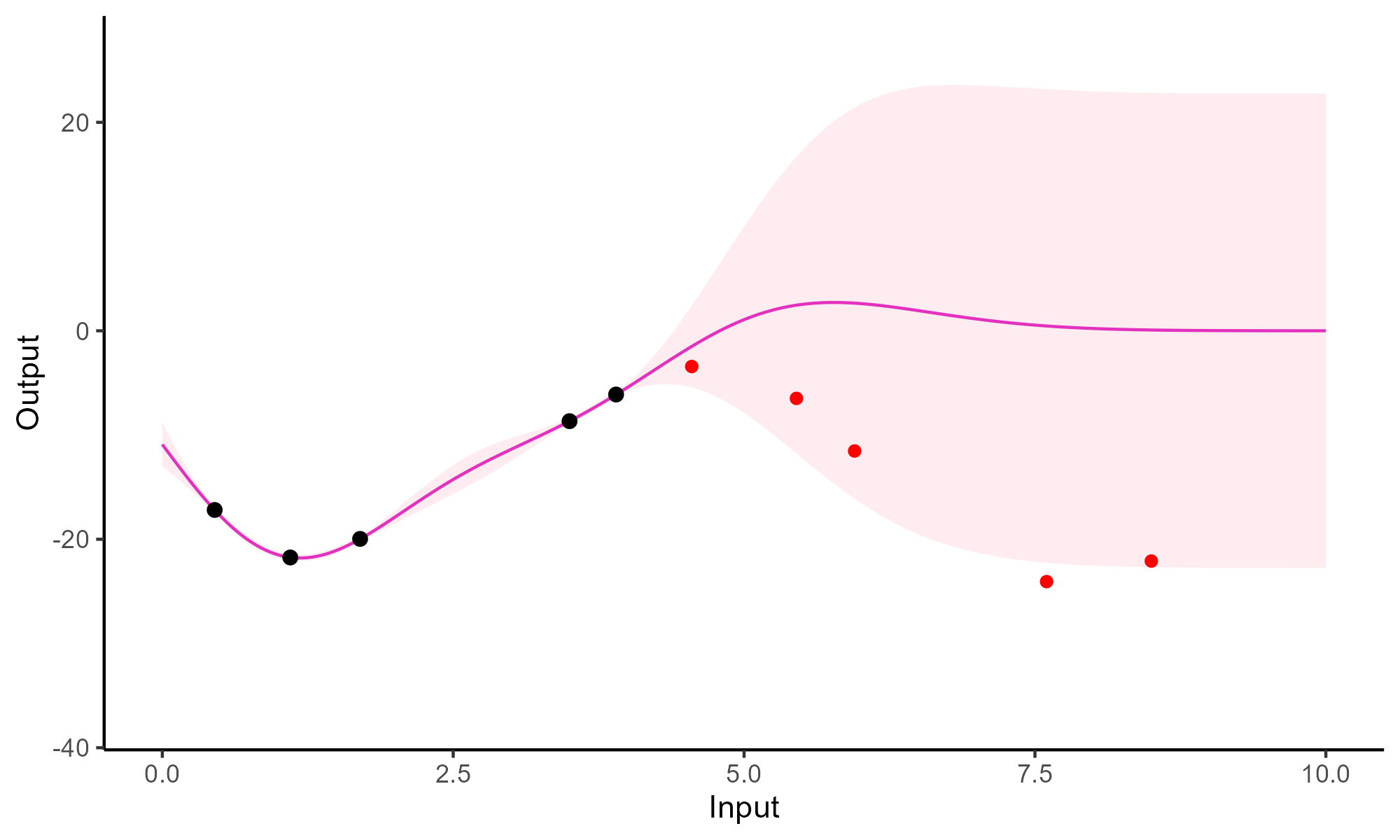
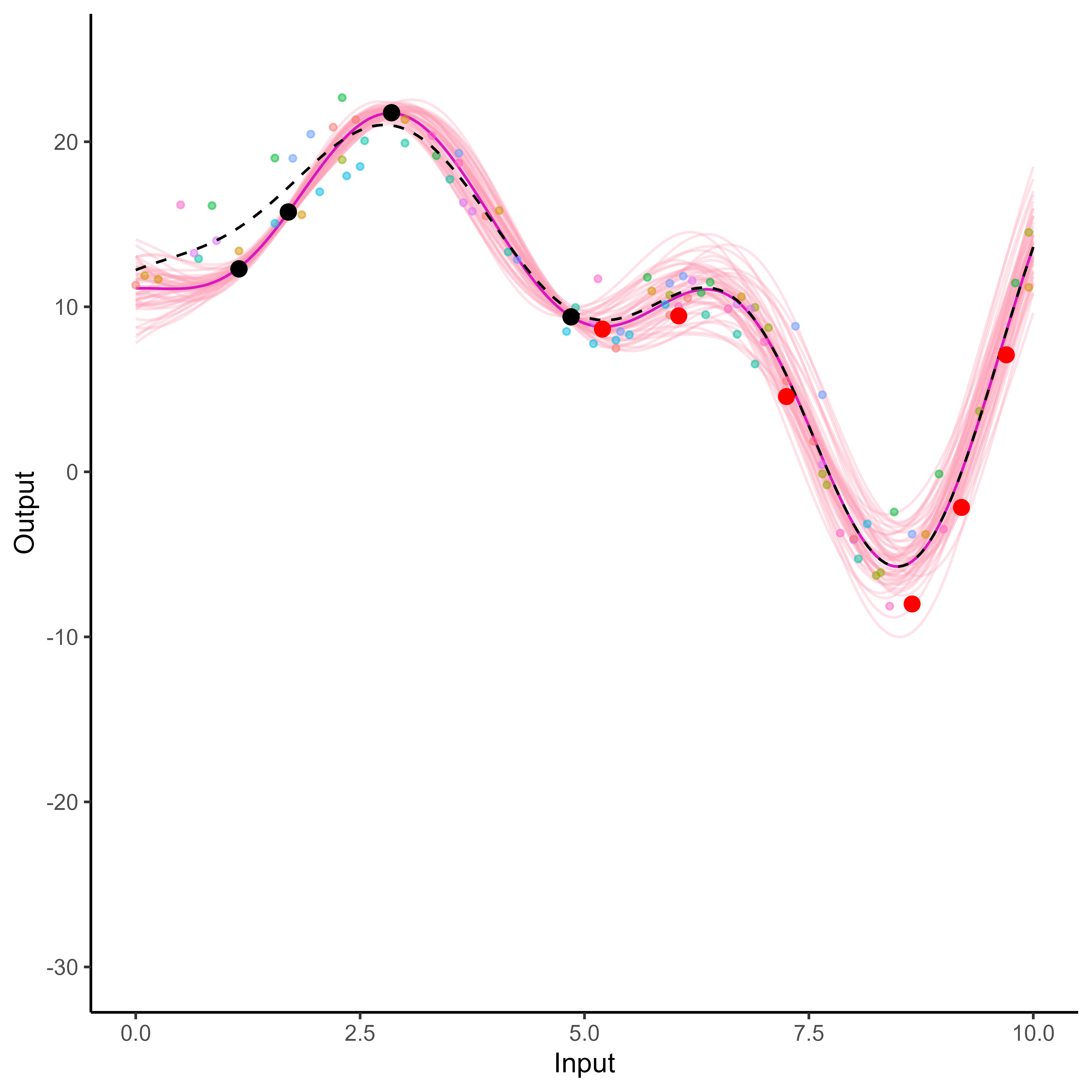
Prediction: updating our knowledge about functions

\(f_{\color{purple}{m}} \mid f_{\color{grey}{o}} \sim \mathcal{N} \Big( m_{\color{purple}{m}} + C_{\color{purple}{m}, \color{grey}{o}} C_{\color{grey}{o, o}}^{-1} (f_{\color{grey}{o}} - m_{\color{grey}{o}}), \ \ C_{\color{purple}{m, m}} - C_{\color{purple}{m}, \color{grey}{o}} C_{\color{grey}{o, o}}^{-1} C_{\color{grey}{o}, \color{purple}{m}} \Big)\)

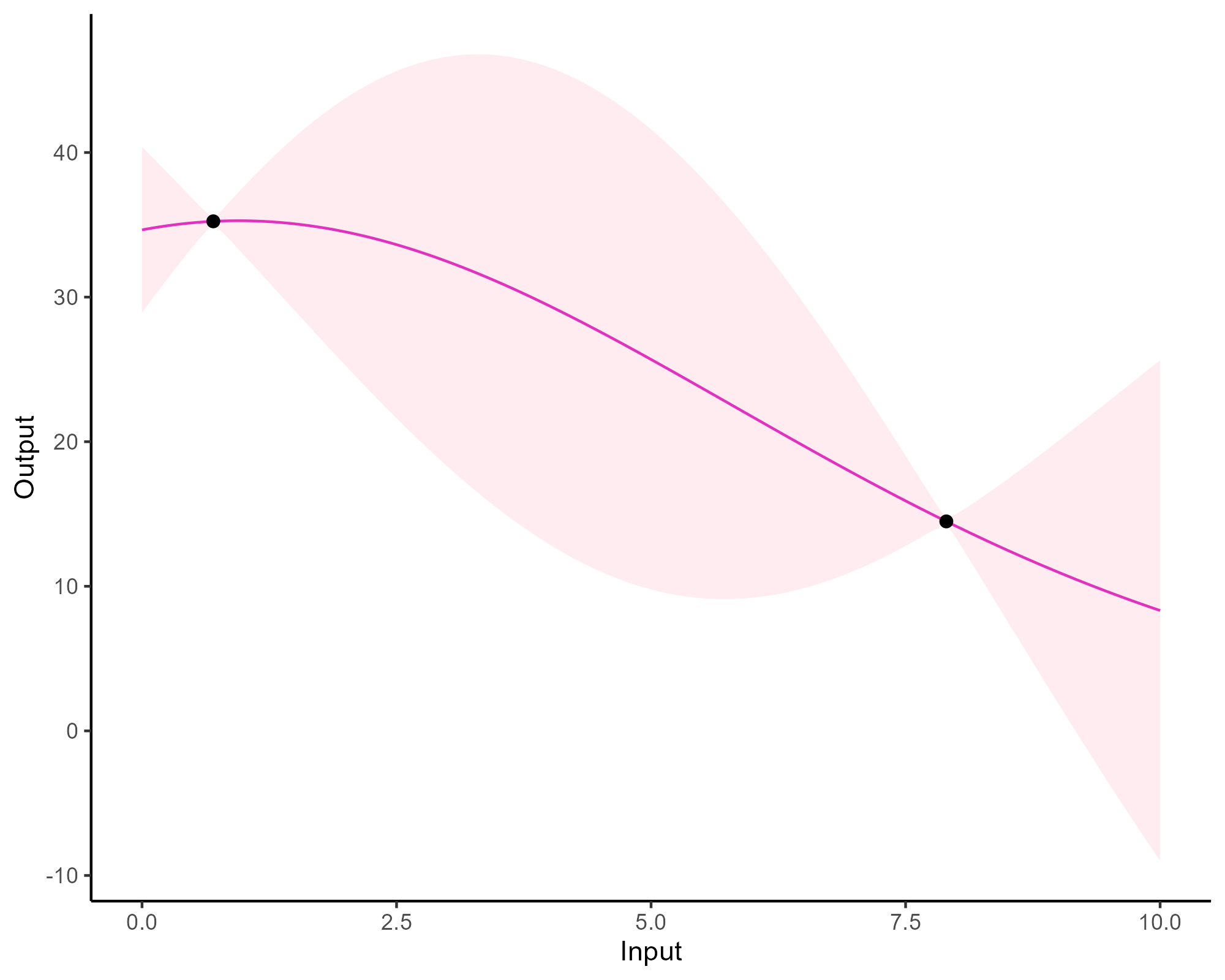
Forecasting with a unique GP

Forecasting with a unique GP

Go play with GPs!

Try and play with the amazing interactive GP visualisation tool available at:

https://www.infinitecuriosity.org/vizgp/

Multi-Task? Multi-Output? What are the maths behind that?

In the previous examples, we saw a variety of situations that naturally lead to the same mathematical formulation of the learning problem:

\[y_s = \color{orange}{f_s}(x_s) + \epsilon_s, \hspace{3cm} \forall s = 1, \dots, S\]

Learn \(\color{orange}{f_s}\), the underlying relationship between \(x_s\) and \(y_s\), for each source of data \(\color{orange}{s}\).

Multi-, in contrast with single-, regression implies that some information can be shared across data sources to improve learning/predictions.

The nature of measurements leads to a more philosophical distinction:

• Multi-Output clearly refers to several variables of interest. An Output is a quantity we aim to infer/predict from Input measurements, and which may be correlated with others.
• Multi-Task implies the existence of an underlying pattern, shared by several tasks or individuals, which can be jointly exploited to build a common model.

A long history of old and modern Multi-Output strategies

• A large litterature in geostatistics, from the origins in the 60s, is known as co-kriging.
• Alvarez et al. - Kernels for Vector-Valued Functions: A Review - Foundations and Trends in Machine Learning, 2011
• Parra and Tobar - Spectral mixture kernels for multi-output Gaussian processes - NeurIPS, 2017
• Liu et al. - Remarks on multi-output Gaussian process regression - Knowledge-Based Systems, 2018
• Bruinsma et al. - Scalable Exact Inference in Multi-Output Gaussian Processes - PMLR, 2020
  
• Van der Wilk et al. - A framework for interdomain and multioutput Gaussian processes - arXiv preprint, 2020

A nice overview of Multi-Output GPs concepts:

• GPSS 2017 video recording - Multi-Output Gaussian Processes - Mauricio Alvarez

Multi-Output GPs: exploiting explicit correlations

Instead of modelling multiple tasks (or individuals, or outputs) independently with a single GPs, we could leverage correlations existing across them.

A natural approach comes from defining multi-output kernels, explicitly modelling correlations between each task-input couple. A classical assumption is separable covariance structures:

\[k\left((i, x),\left(j, x^{\prime}\right)\right)=\operatorname{cov}\left(f_i(x), f_j\left(x^{\prime}\right)\right)=K^{\mathrm{O}}_{i, j} \times k_{\mathrm{I}}\left(x, x^{\prime}\right)\]

By stacking outputs into one vector \(\textbf{y} = \{\textbf{y}_1, \dots, \textbf{y}_M\}^{\intercal}\), the matrices build from those kernels can be represented through a Kronecker product:

\[\textbf{K} = \textbf{K}^{\mathrm{O}} \otimes \textbf{K}_{\mathrm{I}}\]

There exist many ways to define multi-output kernels, we will see a brief overview of a few important ones. In practice, it can be difficult to learn explicit inter-task correlations (i.e. the elements of \(\boldsymbol{K^{\mathrm{O}}}\)) from data, with a computational complexity for exact training of \(\mathcal{O}(\color{red}{O}^3N^3)\).

Multi-Output GPs: the ideal case

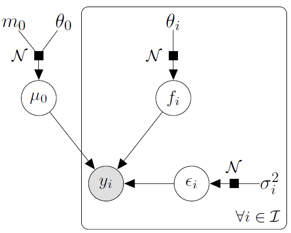
Another paradigm: Multi-Task GPs with shared mean process

\[y_t = \mu_0 + f_t + \epsilon_t, \hspace{3cm} \forall t = 1, \dots, T\]

with:

• \(\mu_0 \sim \mathcal{GP}(m_0, K_{0}),\)
• \(f_t \sim \mathcal{GP}(0, \Sigma_{\theta_t}), \ \perp \!\!\! \perp_t,\)
• \(\epsilon_t \sim \mathcal{GP}(0, \sigma_t^2), \ \perp \!\!\! \perp_t.\)

It follows that:

\[y_t \mid \mu_0 \sim \mathcal{GP}(\mu_0, \Sigma_{\theta_t} + \sigma_t^2 I), \ \perp \!\!\! \perp_t\]

\(\rightarrow\) Unified GP framework with a shared mean process \(\mu_0\), and task-specific process \(f_t\),
\(\rightarrow\) Naturaly handles irregular grids of input data.

Goal: Learn the hyper-parameters, (and \(\mu_0\)’s hyper-posterior).
Difficulty: The likelihood depends on \(\mu_0\), and tasks are not independent.

EM algorithm

E-step

\[ \begin{align} p(\mu_0(\color{grey}{\mathbf{x}}) \mid \textbf{y}, \hat{\Theta}) &\propto \mathcal{N}(\mu_0(\color{grey}{\mathbf{x}}); m_0(\color{grey}{\textbf{x}}), \textbf{K}_{0}^{\color{grey}{\textbf{x}}}) \times \prod\limits_{t =1}^T \mathcal{N}(\mathbf{y}_t; \mu_0( \color{purple}{\textbf{x}_i}), \boldsymbol{\Psi}_{\hat{\theta}_i, \hat{\sigma}_i^2}^{\color{purple}{\textbf{x}_i}}) \\ &= \mathcal{N}(\mu_0(\color{grey}{\mathbf{x}}); \hat{m}_0(\color{grey}{\textbf{x}}), \hat{\textbf{K}}^{\color{grey}{\textbf{x}}}), \end{align} \]

• \(\hat{\textbf{K}}^{\color{grey}{\textbf{x}}} = ({\textbf{K}_{0}^{\color{grey}{\textbf{x}}}}^{-1} + \sum\limits_{t = 1}^T {\boldsymbol{\Psi}_{\hat{\theta}_i, \hat{\sigma}_i^2}^{\color{purple}{\textbf{x}_i}}}^{-1})^{-1}\)
• \(\hat{m}_0(\color{grey}{\textbf{x}}) = \hat{\textbf{K}}^{\color{grey}{\textbf{x}}}({\textbf{K}_{0}^{\color{grey}{\textbf{x}}}}^{-1} m_0(\color{grey}{\mathbf{x}}) + \sum\limits_{t = 1}^T {\boldsymbol{\Psi}_{\hat{\theta}_i, \hat{\sigma}_i^2}^{\color{purple}{\textbf{x}_i}}}^{-1} \mathbf{y}_t)\).

M-step

\[ \begin{align*} \hat{\Theta} &= \underset{\Theta}{\arg\max} \ \ \sum\limits_{t = 1}^{T}\left\{ \log \mathcal{N} \left( \mathbf{y}_t; \hat{m}_0(\color{purple}{\mathbf{x}_t}), \boldsymbol{\Psi}_{\theta_t, \sigma^2}^{\color{purple}{\mathbf{x}_t}} \right) - \dfrac{1}{2} Tr \left( \hat{\mathbf{K}}^{\color{purple}{\mathbf{x}_t}} {\boldsymbol{\Psi}_{\theta_t, \sigma^2}^{\color{purple}{\mathbf{x}_t}}}^{-1} \right) \right\}. \end{align*} \]

Covariance structure assumption and computational complexity

Sharing the covariance structures or not offers a compromise between flexibility and parsimony:

• One optimisation problem for \(\theta\), and a shared process for all tasks,
  
• \(\color{blue}{T}\) distinct optimisation problems for \(\{\theta_t\}_t\), and task-specific processes.

• Both approaches scale linearly with the number of tasks,
  
• Parallel computing can be used to speed up training.

Overall, the computational complexity is: \[ \mathcal{O}(\color{blue}{T} \times N_t^3 + N^3) \]

with \(N = \bigcup\limits_{t = 1}^\color{blue}{T} N_t\)

Prediction

For a new task, we observe some data \(y_*(\textbf{x}_*)\). Let us recall:

\[y_* \mid \mu_0 \sim \mathcal{GP}(\mu_0, \boldsymbol{\Psi}_{\theta_*, \sigma_*^2}), \ \perp \!\!\! \perp_t\]

Goals:

• derive a analytical predictive distribution at arbitrary inputs \(\mathbf{x}^{p}\),
• sharing the information from training tasks, stored in the mean process \(\mu_0\).

Difficulties:

• the model is conditionned over \(\mu_0\), a latent, unobserved quantity,
• defining the adequate target distribution is not straightforward,
• working on a new grid of inputs \(\mathbf{x}^{p}_{*}= (\mathbf{x}_{*}, \mathbf{x}^{p})^{\intercal},\) potentially distinct from \(\mathbf{x}.\)

Prediction: the key idea

Defining a multi-task prior distribution by:

• conditioning on training data,
• integrating over \(\mu_0\)’s hyper-posterior distribution.

\[\begin{align} p(y_* (\textbf{x}_*^{p}) \mid \textbf{y}) &= \int p\left(y_* (\textbf{x}_*^{p}) \mid \textbf{y}, \mu_0(\textbf{x}_*^{p})\right) p(\mu_0 (\textbf{x}_*^{p}) \mid \textbf{y}) \ d \mu_0(\mathbf{x}^{p}_{*}) \\ &= \int \underbrace{ p \left(y_* (\textbf{x}_*^{p}) \mid \mu_0 (\textbf{x}_*^{p}) \right)}_{\mathcal{N}(y_*; \mu_0, \Psi_*)} \ \underbrace{p(\mu_0 (\textbf{x}_*^{p}) \mid \textbf{y})}_{\mathcal{N}(\mu_0; \hat{m}_0, \hat{K})} \ d \mu_0(\mathbf{x}^{p}_{*}) \\ &= \mathcal{N}( \hat{m}_0 (\mathbf{x}^{p}_{*}), \underbrace{\Psi_* + \hat{K}}_{\Gamma}) \end{align}\]

Final prediction: the good old GP formula

• Multi-Task prior:

\[p \left( \begin{bmatrix} y_*(\color{grey}{\mathbf{x}_{*}}) \\ y_*(\color{purple}{\mathbf{x}^{p}}) \\ \end{bmatrix} \mid \textbf{y} \right) = \mathcal{N} \left( \begin{bmatrix} y_*(\color{grey}{\mathbf{x}_{*}}) \\ y_*(\color{purple}{\mathbf{x}^{p}}) \\ \end{bmatrix}; \ \begin{bmatrix} \hat{m}_0(\color{grey}{\mathbf{x}_{*}}) \\ \hat{m}_0(\color{purple}{\mathbf{x}^{p}}) \\ \end{bmatrix}, \begin{pmatrix} \Gamma_{\color{grey}{**}} & \Gamma_{\color{grey}{*}\color{purple}{p}} \\ \Gamma_{\color{purple}{p}\color{grey}{*}} & \Gamma_{\color{purple}{pp}} \end{pmatrix} \right)\]

• Multi-Task posterior:

\[p(y_*(\color{purple}{\mathbf{x}^{p}}) \mid y_*(\color{grey}{\mathbf{x}_{*}}), \textbf{y}) = \mathcal{N} \Big( y_*(\color{purple}{\mathbf{x}^{p}}); \ \hat{\mu}_{*}(\color{purple}{\mathbf{x}^{p}}) , \hat{\Gamma}_{\color{purple}{pp}} \Big)\]

with:

• \(\hat{\mu}_{*}(\color{purple}{\mathbf{x}^{p}}) = \hat{m}_0(\color{purple}{\mathbf{x}^{p}}) + \Gamma_{\color{purple}{p}\color{grey}{*}}\Gamma_{\color{grey}{**}}^{-1} (y_*(\color{grey}{\mathbf{x}_{*}}) - \hat{m}_0 (\color{grey}{\mathbf{x}_{*}}))\)
• \(\hat{\Gamma}_{\color{purple}{pp}} = \Gamma_{\color{purple}{pp}} - \Gamma_{\color{purple}{p}\color{grey}{*}}\Gamma_{\color{grey}{**}}^{-1} \Gamma_{\color{grey}{*}\color{purple}{p}}\)

A GIF is worth a thousand words

A GIF is worth a thousand words

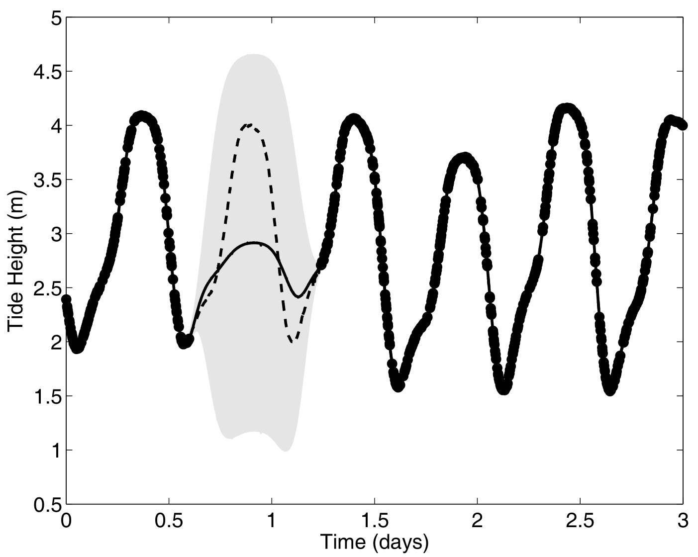
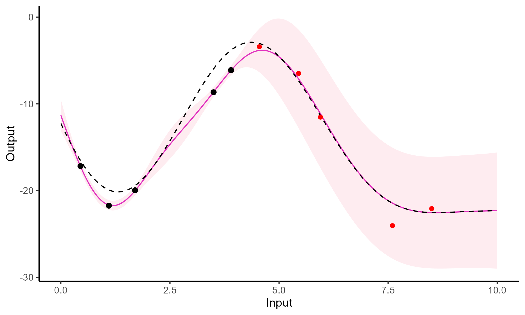
Comparison with single GP regression

What happens with multi-dimensional inputs?

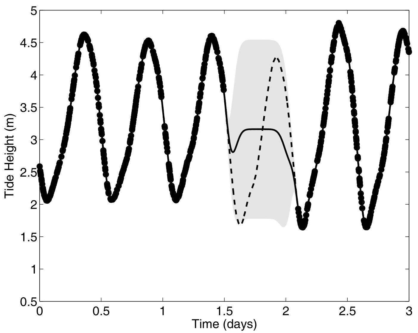
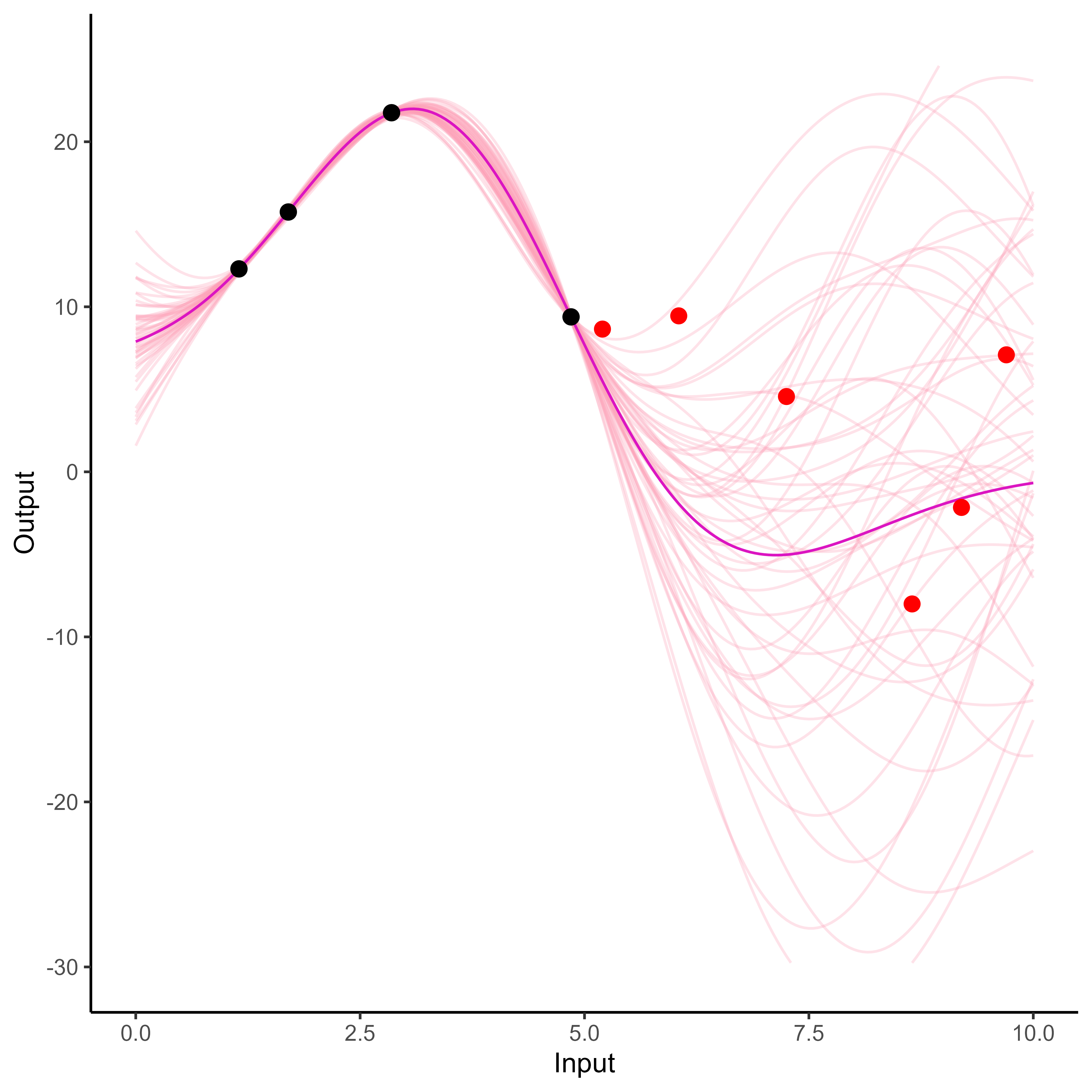
Yet another comparison with single GP regression

Multi-Task GPs regression provides more reliable predictions when individual processes are sparsely observed, while greatly reducing the associated uncertainty

Adding some clustering into Multi-Task GPs

A unique underlying mean process might be too restrictive.

\(\rightarrow\) Mixture of multi-task GPs:

\[y_t = \mu_0 + f_t + \epsilon_t, \hspace{3cm} \forall t = 1, \dots, T\]

with:

• \(\color{green}{Z_{t}} \sim \mathcal{M}(1, \color{green}{\boldsymbol{\pi}}), \ \perp \!\!\! \perp_t,\)

• \(\mu_0 \sim \mathcal{GP}(m_0, K_0),\)
• \(f_t \sim \mathcal{GP}(0, \Sigma_{\theta_t}), \ \perp \!\!\! \perp_t,\)
• \(\epsilon_t \sim \mathcal{GP}(0, \sigma_t^2), \ \perp \!\!\! \perp_t.\)

It follows that:

\[y_t \mid \mu_0 \sim \mathcal{GP}(\mu_0, \Psi_t), \ \perp \!\!\! \perp_t\]

Adding some clustering into Multi-Task GPs

A unique underlying mean process might be too restrictive.

\(\rightarrow\) Mixture of multi-task GPs:

\[y_t \mid \{\color{green}{Z_{tk}} = 1 \} = \mu_{\color{green}{k}} + f_t + \epsilon_t, \hspace{3cm} \forall t = 1, \dots, T\]

with:

• \(\color{green}{Z_{t}} \sim \mathcal{M}(1, \color{green}{\boldsymbol{\pi}}), \ \perp \!\!\! \perp_t,\)
• \(\mu_{\color{green}{k}} \sim \mathcal{GP}(m_{\color{green}{k}}, \color{green}{C_{{k}}})\ \perp \!\!\! \perp_{\color{green}{k}},\)
• \(f_t \sim \mathcal{GP}(0, \Sigma_{\theta_t}), \ \perp \!\!\! \perp_t,\)
• \(\epsilon_t \sim \mathcal{GP}(0, \sigma_t^2), \ \perp \!\!\! \perp_t.\)

It follows that:

\[y_t \mid \mu_0 \sim \mathcal{GP}(\mu_0, \Psi_t), \ \perp \!\!\! \perp_t\]

Adding some clustering into Multi-Task GPs

A unique underlying mean process might be too restrictive.

\(\rightarrow\) Mixture of multi-task GPs:

\[y_t \mid \{\color{green}{Z_{ik}} = 1 \} = \mu_{\color{green}{k}} + f_t + \epsilon_t, \hspace{3cm} \forall t = 1, \dots, T\]

with:

• \(\color{green}{Z_{t}} \sim \mathcal{M}(1, \color{green}{\boldsymbol{\pi}}), \ \perp \!\!\! \perp_t,\)
• \(\mu_{\color{green}{k}} \sim \mathcal{GP}(m_{\color{green}{k}}, \color{green}{C_{{k}}})\ \perp \!\!\! \perp_{\color{green}{k}},\)
• \(f_t \sim \mathcal{GP}(0, \Sigma_{\theta_t}), \ \perp \!\!\! \perp_t,\)
• \(\epsilon_t \sim \mathcal{GP}(0, \sigma_t^2), \ \perp \!\!\! \perp_t.\)

It follows that:

\[y_t \mid \{ \boldsymbol{\mu} , \color{green}{\boldsymbol{\pi}} \} \sim \sum\limits_{k=1}^K{ \color{green}{\pi_k} \ \mathcal{GP}\Big(\mu_{\color{green}{k}}, \Psi_t^\color{green}{k} \Big)}, \ \perp \!\!\! \perp_t\]

Variational EM

E step: \[ \begin{align} \hat{q}_{\boldsymbol{\mu}}(\boldsymbol{\mu}) &= \color{green}{\prod\limits_{k = 1}^K} \mathcal{N}(\mu_\color{green}{k};\hat{m}_\color{green}{k}, \hat{\textbf{C}}_\color{green}{k}) , \hspace{2cm} \hat{q}_{\boldsymbol{Z}}(\boldsymbol{Z}) = \prod\limits_{t = 1}^T \mathcal{M}(Z_t;1, \color{green}{\boldsymbol{\tau}_t}) \end{align} \] M step:

\[ \begin{align*} \hat{\Theta} &= \underset{\Theta}{\arg\max} \sum\limits_{k = 1}^{K}\sum\limits_{t = 1}^{T}\tau_{tk}\ \mathcal{N} \left( \mathbf{y}_t; \ \hat{m}_k, \boldsymbol{\Psi}_{\color{blue}{\theta_t}, \color{blue}{\sigma_t^2}} \right) - \dfrac{1}{2} \textrm{tr}\left( \mathbf{\hat{C}}_k\boldsymbol{\Psi}_{\color{blue}{\theta_t}, \color{blue}{\sigma_t^2}}^{-1}\right) \\ & \hspace{1cm} + \sum\limits_{k = 1}^{K}\sum\limits_{t = 1}^{T}\tau_{tk}\log \color{green}{\pi_{k}} \end{align*} \]

Cluster-specific and mixture predictions

• Multi-Task posterior for each cluster:

\[ p(y_*(\mathbf{x}^{p}) \mid \color{green}{Z_{*k}} = 1, y_*(\mathbf{x}_{*}), \textbf{y}) = \mathcal{N} \Big( y_*(\mathbf{x}^{p}); \ \hat{\mu}_{*}^\color{green}{k}(\mathbf{x}^{p}) , \hat{\Gamma}_{pp}^\color{green}{k} \Big), \forall \color{green}{k}, \]

\(\hat{\mu}_{*}^\color{green}{k}(\mathbf{x}^{p}) = \hat{m}_\color{green}{k}(\mathbf{x}^{p}) + \Gamma^\color{green}{k}_{p*} {\Gamma^\color{green}{k}_{**}}^{-1} (y_*(\mathbf{x}_{*}) - \hat{m}_\color{green}{k} (\mathbf{x}_{*}))\)
\(\hat{\Gamma}_{pp}^\color{green}{k} = \Gamma_{pp}^\color{green}{k} - \Gamma_{p*}^\color{green}{k} {\Gamma^{\color{green}{k}}_{**}}^{-1} \Gamma^{\color{green}{k}}_{*p}\)

• Predictive multi-task GPs mixture:

\[p(y_*(\textbf{x}^p) \mid y_*(\textbf{x}_*), \textbf{y}) = \color{green}{\sum\limits_{k = 1}^{K} \tau_{*k}} \ \mathcal{N} \big( y_*(\mathbf{x}^{p}); \ \hat{\mu}_{*}^\color{green}{k}(\textbf{x}^p) , \hat{\Gamma}_{pp}^\color{green}{k}(\textbf{x}^p) \big).\]

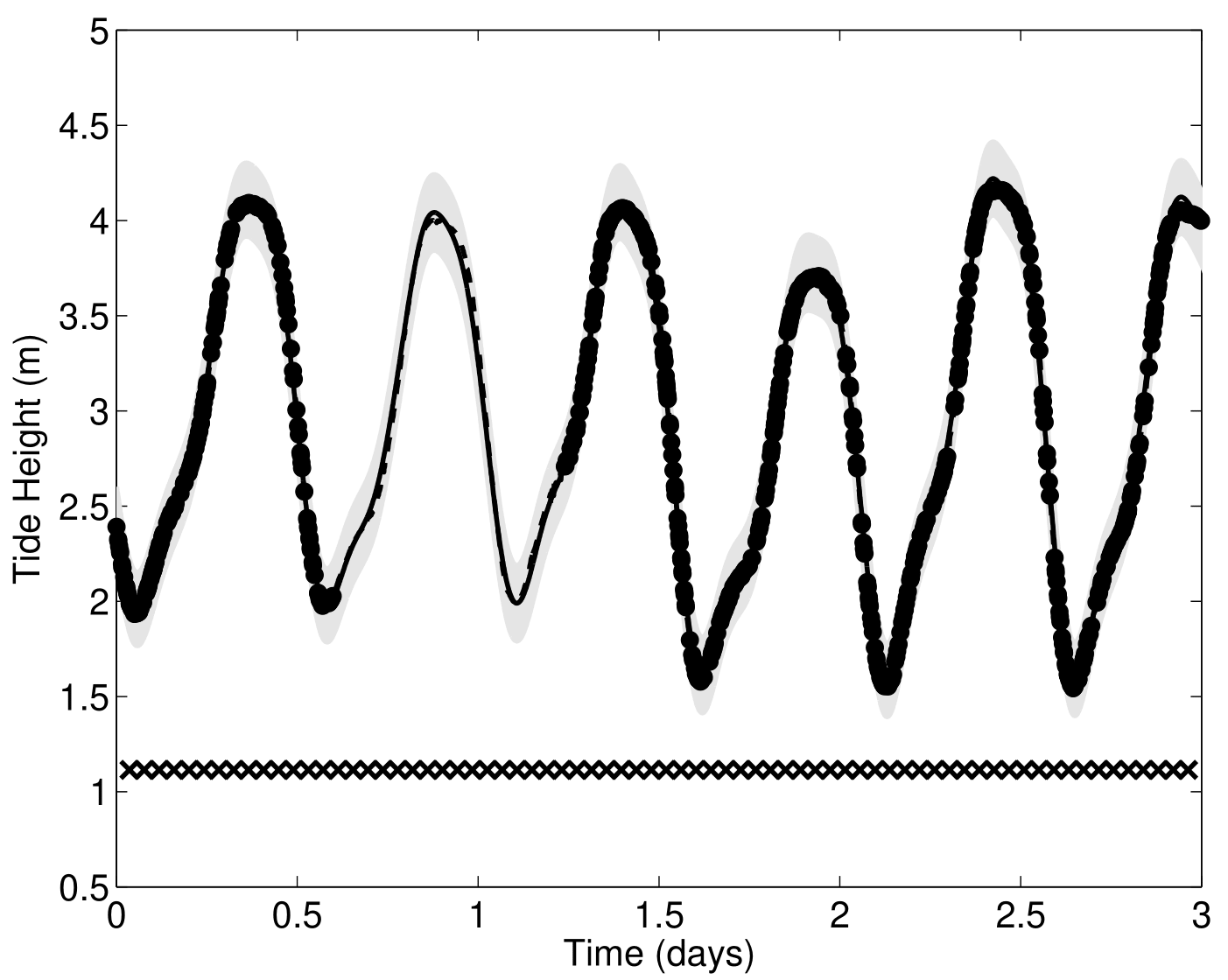
An image is still worth many words

A unique mean process can struggle to capture relevant signals in presence of group structures.

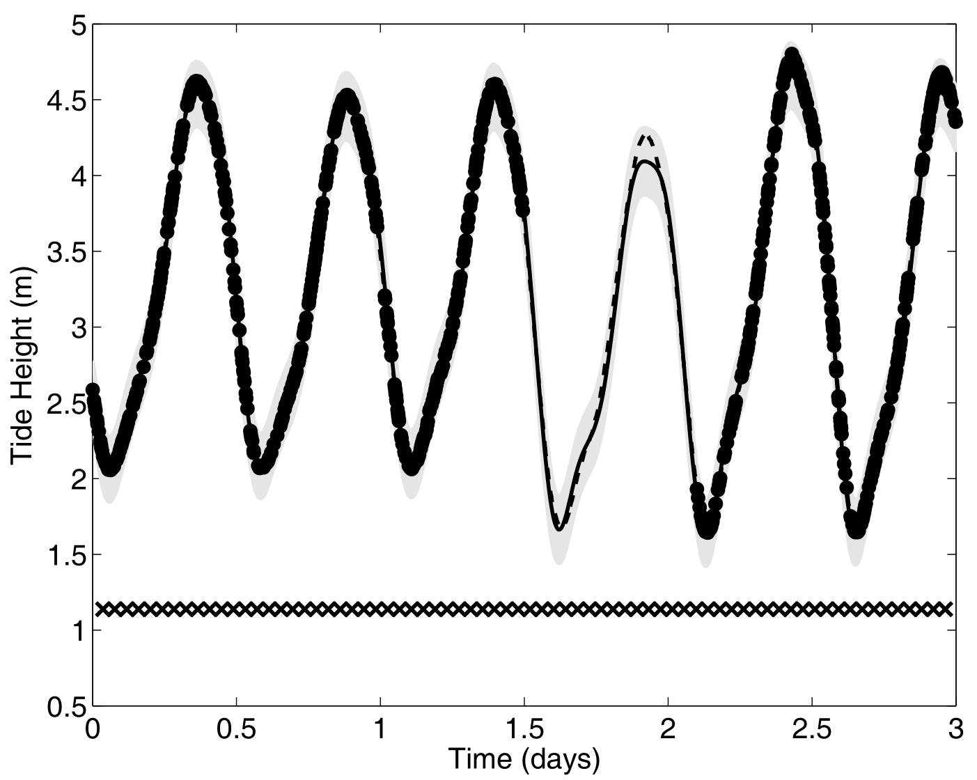
An image is still worth many words

By identifying the underlying clustering structure, we can discard unnecessary information and provide enhanced predictions as well as lower uncertainty.

Saved by the weights

Each cluster-specific prediction is weighted by its membership probability \(\color{green}{\tau_{*k}}\).

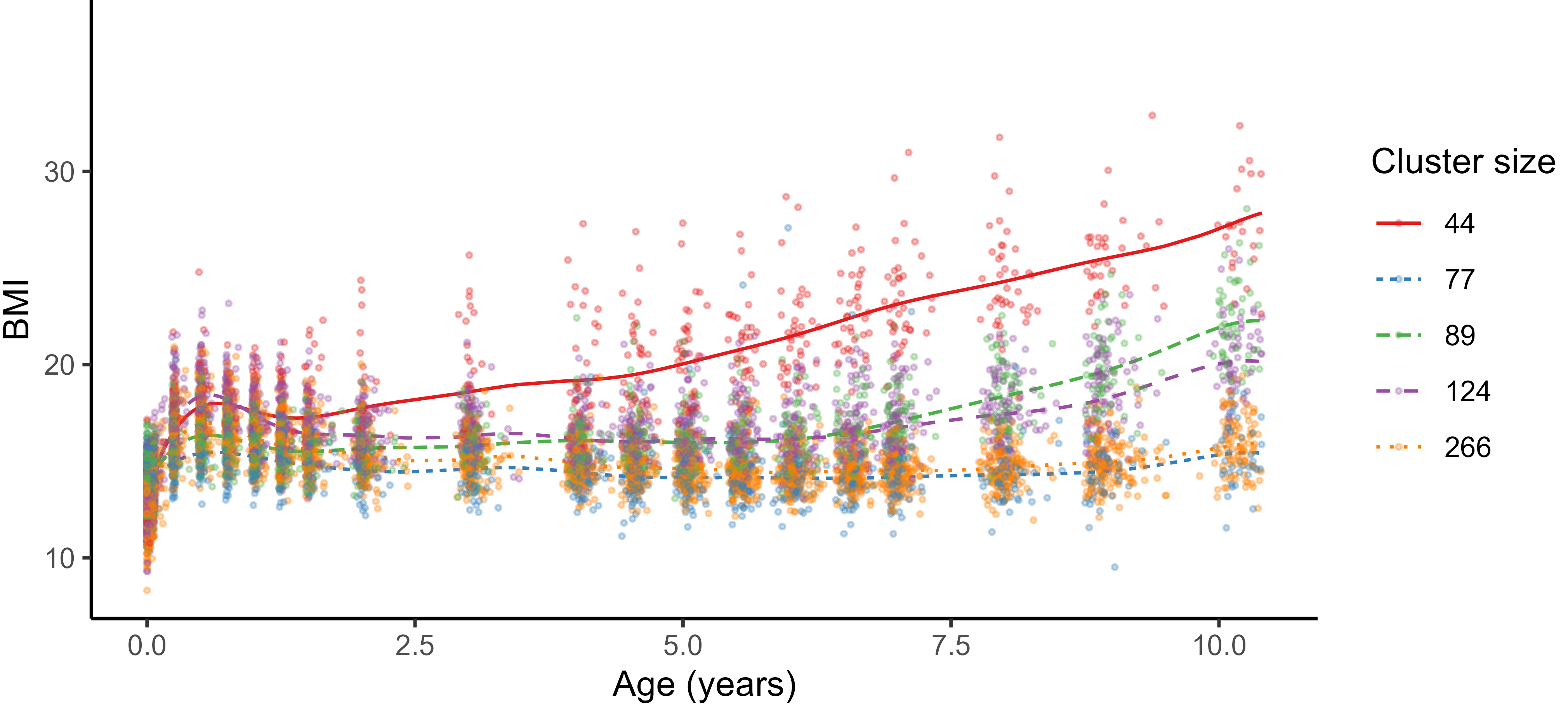
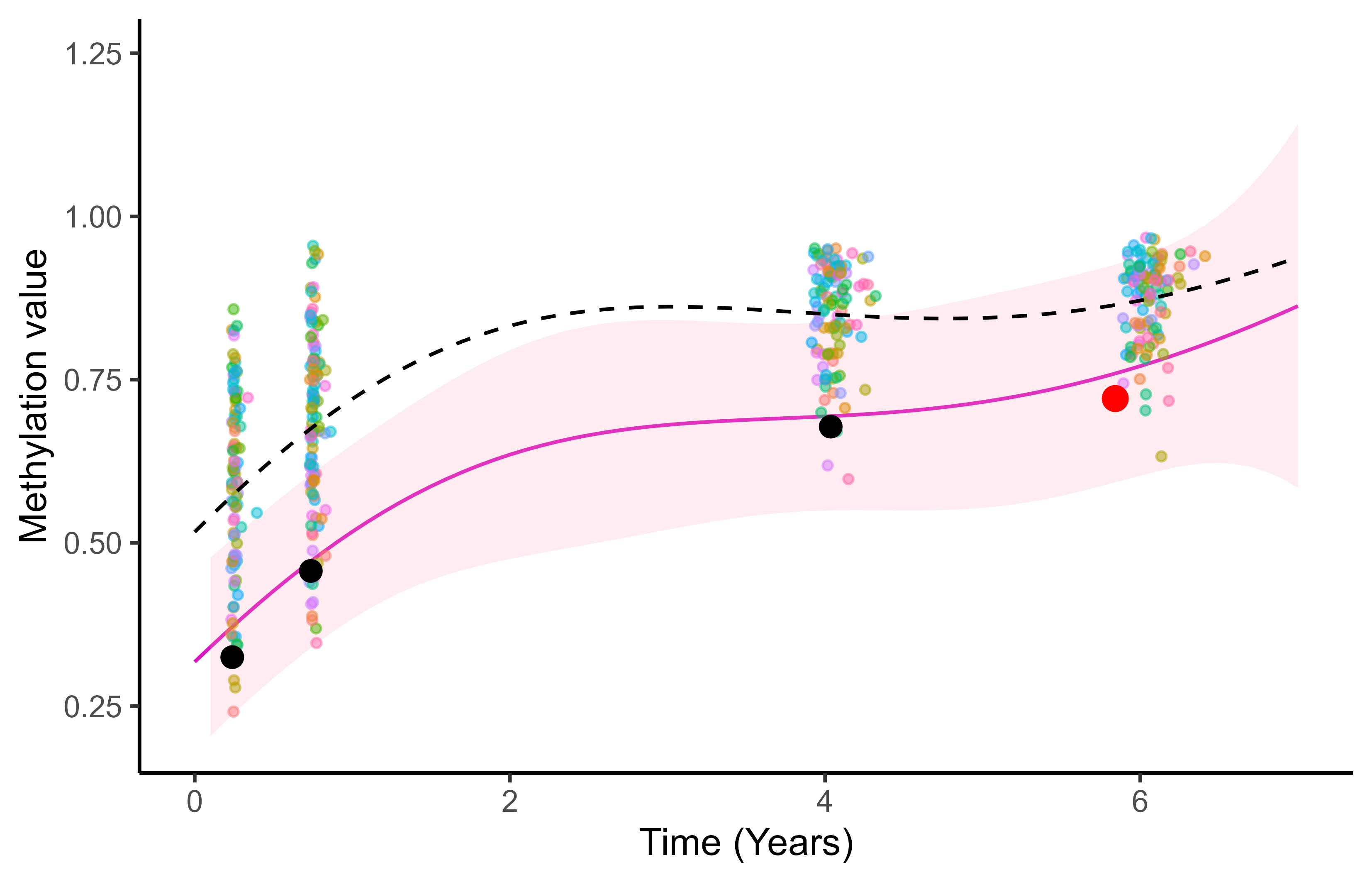
Practical application: follow up of BMI during childhood

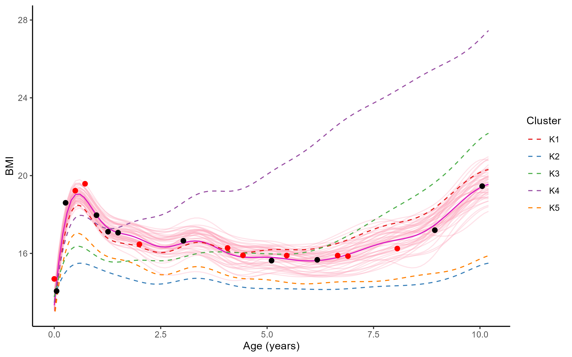
Reconstruction for sparse or incomplete data

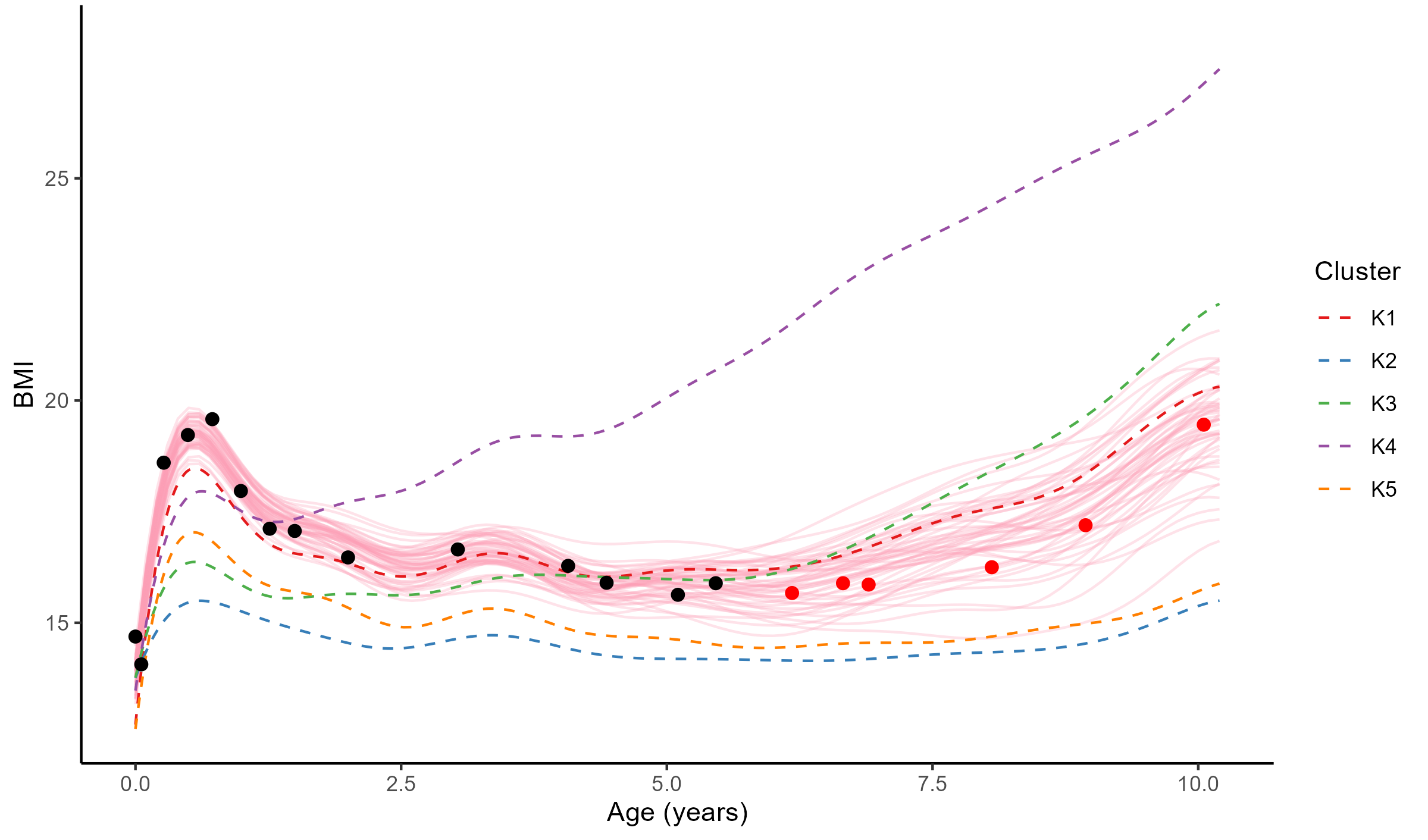
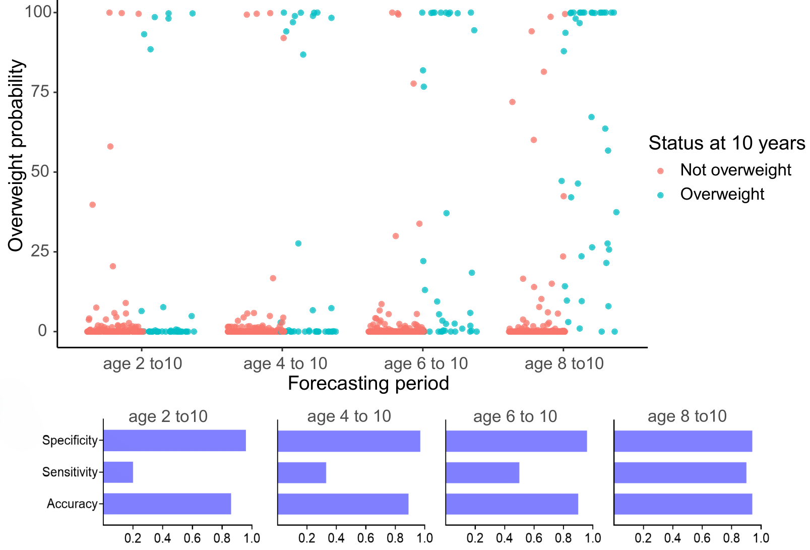
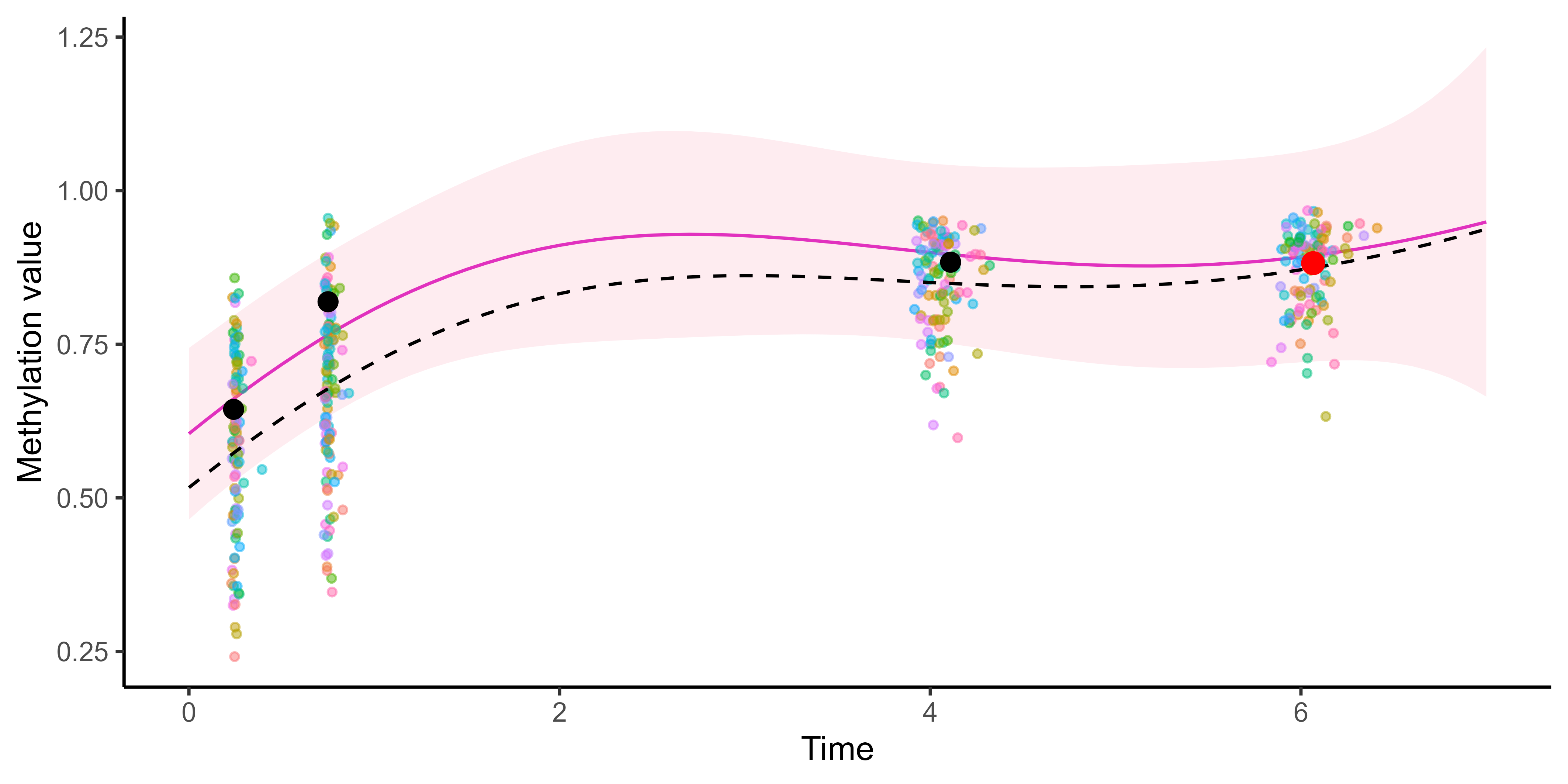
Forecasting long term evolution of BMI

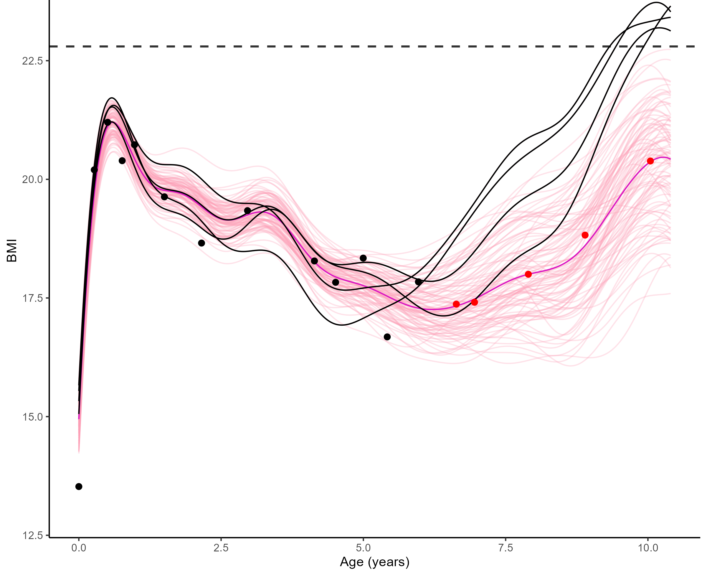
Leveraging the uncertainty quantification of GPs

Deriving downstream tools for practitioners

Uncertainty quantification provides valuable information to practitioners to make decisions based on probabilistic statements, like the risk of overweight at 10 years.

Feel free to test it on your data

Implemented as an R package MagmaClustR: https://arthurleroy.github.io/MagmaClustR

Multi-Task-Multi-Output GPs: best of both worlds?

We have reviewed two different paradigms to tackle an identical mathematical problem:

• Multi-Output GPs derive full rank covariance matrices to exploit cross-correlations between all Input-Output pairs. They are flexible, expressive, and well-designed to recover very different signals or measurements. On the down side, they are computationally expensive, sometimes difficult to train in practice, and poorly adapted to modelling multiple tasks/individuals.

• Multi-Task GPs leverage latent mean processes to share information on the common trends and properties of the data. They are parsimonious, efficient, and well-designed to capture common patterns for multiple tasks/individuals on the same variable of interest. On the down side, they can be limited to fully capture correlations between the GPs and exploit initial knowledge that collected data may be of different natures.

Both work on separate parts of a GP, with no assumption on the other, and are theoretically compatible. They are even expected to synergise well, by tackling each others limitations.

Generative model of MOMT GPs

\[\begin{bmatrix} y_t^{1} \\ \vdots \\ y_t^{O} \\ \end{bmatrix} = \begin{bmatrix} \mu_0 \\ \vdots \\ \mu_0 \\ \end{bmatrix} + \begin{bmatrix} f_t^{1} \\ \vdots \\ f_t^{O} \\ \end{bmatrix} + \begin{bmatrix} \epsilon_t^{1} \\ \vdots \\ \epsilon_t^{O} \\ \end{bmatrix}, \hspace{3cm} \forall t = 1, \dots, T\]

• \(\mu_0 \sim \mathcal{GP}(m_0, K_0),\)
• \(\begin{bmatrix} f_t^{1} \\ \vdots \\ f_t^{O} \\ \end{bmatrix} \sim \mathcal{GP}(0, \Sigma_{\theta_t}), \ \perp \!\!\! \perp_t,\)
• \(\begin{bmatrix} \epsilon_t^{1} \\ \vdots \\ \epsilon_t^{O} \\ \end{bmatrix} \sim \mathcal{GP}(0, \begin{bmatrix} {\sigma_t^{1}}^O \\ \vdots \\ {\sigma_{t}^O}^2 \\ \end{bmatrix} \times I_O), \ \perp \!\!\! \perp_t.\)

All mathematical objects from Multi-Task GPs are now extended with stacked Outputs.

Process convolution covariance structure and inference

\[\Big[k_{\theta_t}(\mathbf{x}, \mathbf{x}^{\prime})\Big]_{o,o'} = \dfrac{S_{t,o} \ S_{t,o{\prime}}}{(2\pi)^{D/2} \ |\Sigma|^{1/2}} \ \exp\Big(-\dfrac{1}{2}(\mathbf{x} - \mathbf{x}^{\prime})^T \Sigma^{-1}(\mathbf{x}-\mathbf{x}^{\prime})\Big)\]

• \(S_{t,o}, S_{t,o{\prime}} \in \mathbb{R}\), the Output-specific variance terms,
• \(\Sigma = P_{t,o}^{-1}+P_{t,o^{\prime}}^{-1}+\Lambda^{-1} \in \mathbb{R}^{D \times D}\).

These matrices are typically diagonal, filled with Output-specific and latent lengthscales, one per Input dimension. In the end, we need to optimise \(\color{red}{O}\times \color{blue}{T} \times (3D+1)\) hyper-parameters.

E-step

\[ \begin{align} p(\mu_0(\color{grey}{\mathbf{x}}) \mid \textbf{y}, \hat{\Theta}) = \mathcal{N}(\mu_0(\color{grey}{\mathbf{x}}); \hat{m}_0(\color{grey}{\textbf{x}}), \hat{\textbf{K}}^{\color{grey}{\textbf{x}}}), \end{align} \]

M-step

\[ \begin{align*} \hat{\Theta} &= \underset{\Theta}{\arg\max} \sum\limits_{t = 1}^{T}\left\{ \log \mathcal{N} \left( \mathbf{y}_t; \hat{m}_0(\color{purple}{\mathbf{x}_t^O}), \boldsymbol{\Psi}_{\theta_t, \sigma_t^2}^{\color{purple}{\mathbf{x}_t^O}} \right) - \dfrac{1}{2} Tr \left( \hat{\mathbf{K}}^{\color{purple}{\mathbf{x}_t^O}} {\boldsymbol{\Psi}_{\theta_t, \sigma_t^2}^{\color{purple}{\mathbf{x}_t^O}}}^{-1} \right) \right\}. \end{align*} \]

Prediction and properties

As before we get a multi-task posterior predictive distribution in closed form:

\[p\left(\begin{bmatrix} y_1^*(\color{purple}{\mathbf{x}^{p}_1}) \\ \vdots \\ y_1^*(\color{purple}{\mathbf{x}^{p}_O}) \\ \end{bmatrix} \mid \begin{bmatrix} y_1^*(\color{grey}{\mathbf{x}_1^*}) \\ \vdots \\ y_1^*(\color{grey}{\mathbf{x}_O^*}) \\ \end{bmatrix}, \textbf{y} \right) = \mathcal{N} \left(\begin{bmatrix} y_1^*(\color{purple}{\mathbf{x}^{p}_1}) \\ \vdots \\ y_1^*(\color{purple}{\mathbf{x}^{p}_O}) \\ \end{bmatrix}; \ \hat{\mu}_{*}(\color{purple}{\mathbf{x}^{p}}) , \hat{\Gamma}_{\color{purple}{pp}} \right)\]

with:

• \(\hat{\mu}_{*}(\color{purple}{\mathbf{x}^{p}_O}) = \hat{m}_0(\color{purple}{\mathbf{x}^{p}_O}) + \Gamma_{\color{purple}{p}\color{grey}{*}}\Gamma_{\color{grey}{**}}^{-1} (y_*(\color{grey}{\mathbf{x}_1^*}) - \hat{m}_0 (\color{grey}{\mathbf{x}_O^*}))\)
• \(\hat{\Gamma}_{\color{purple}{pp}} = \Gamma_{\color{purple}{pp}} - \Gamma_{\color{purple}{p}\color{grey}{*}}\Gamma_{\color{grey}{**}}^{-1} \Gamma_{\color{grey}{*}\color{purple}{p}}\)

• These objects are typically of dimension \(O \times N_p^o\), which corresponds to the grid of target locations over all Outputs, for a particular Task.
• These observation and prediction grids can be irregular across Tasks and Outputs, and are robust to entirely missing Outputs (even an entire Task, with the posterior mean process)

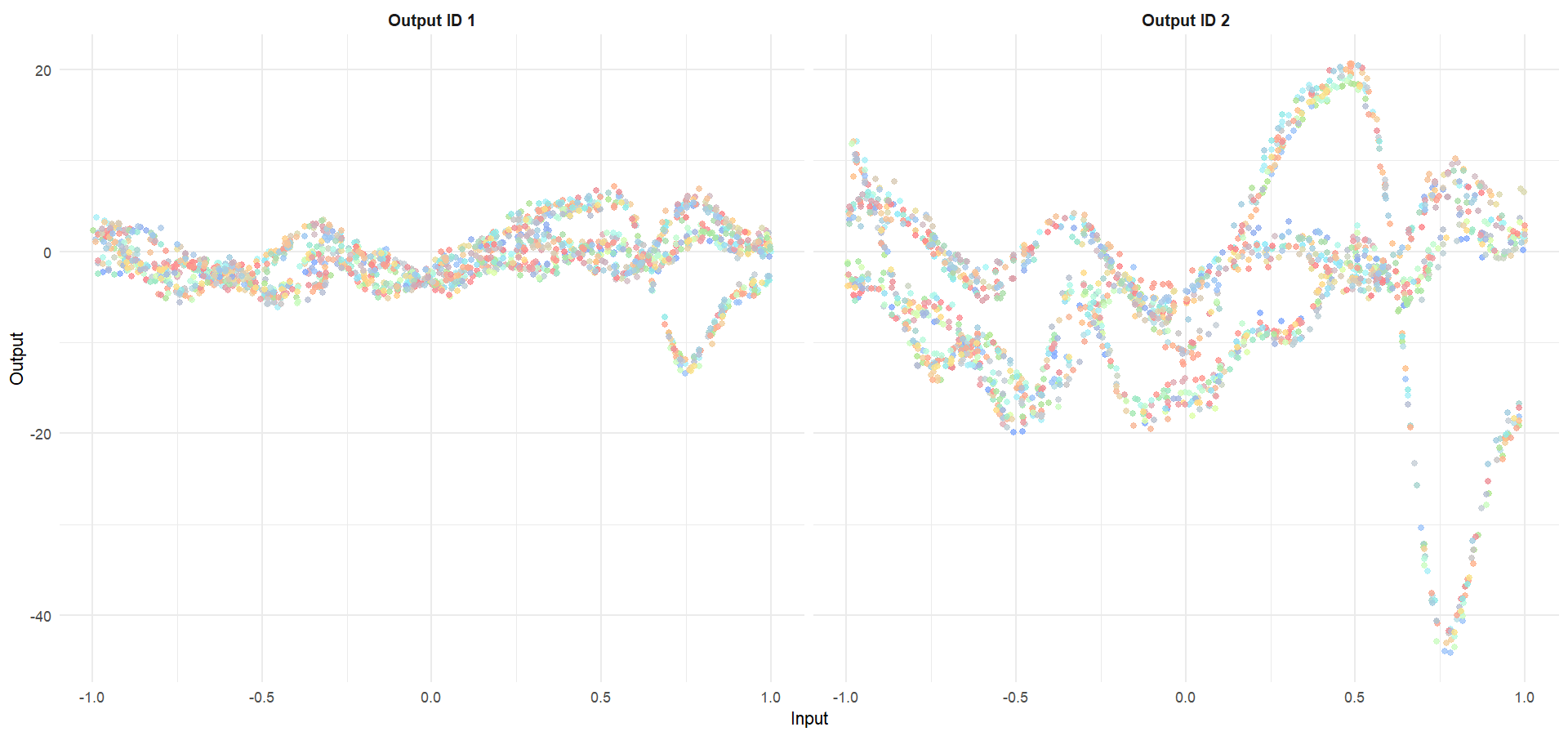
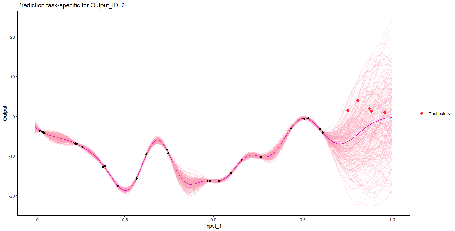
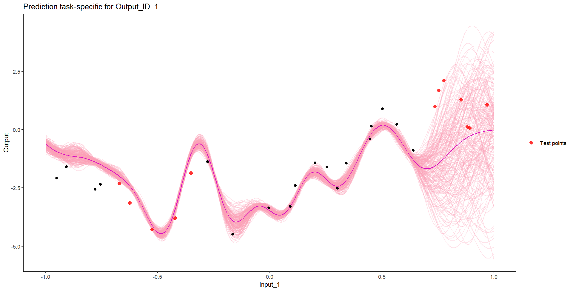
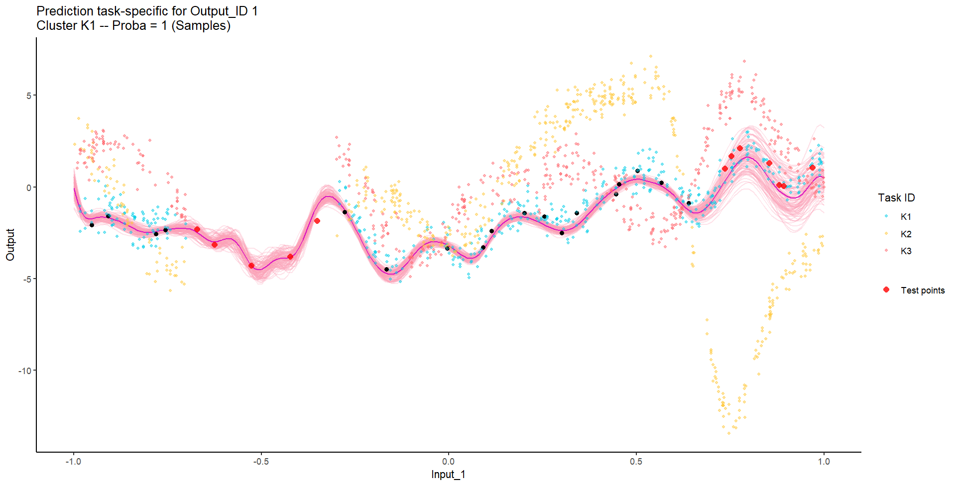
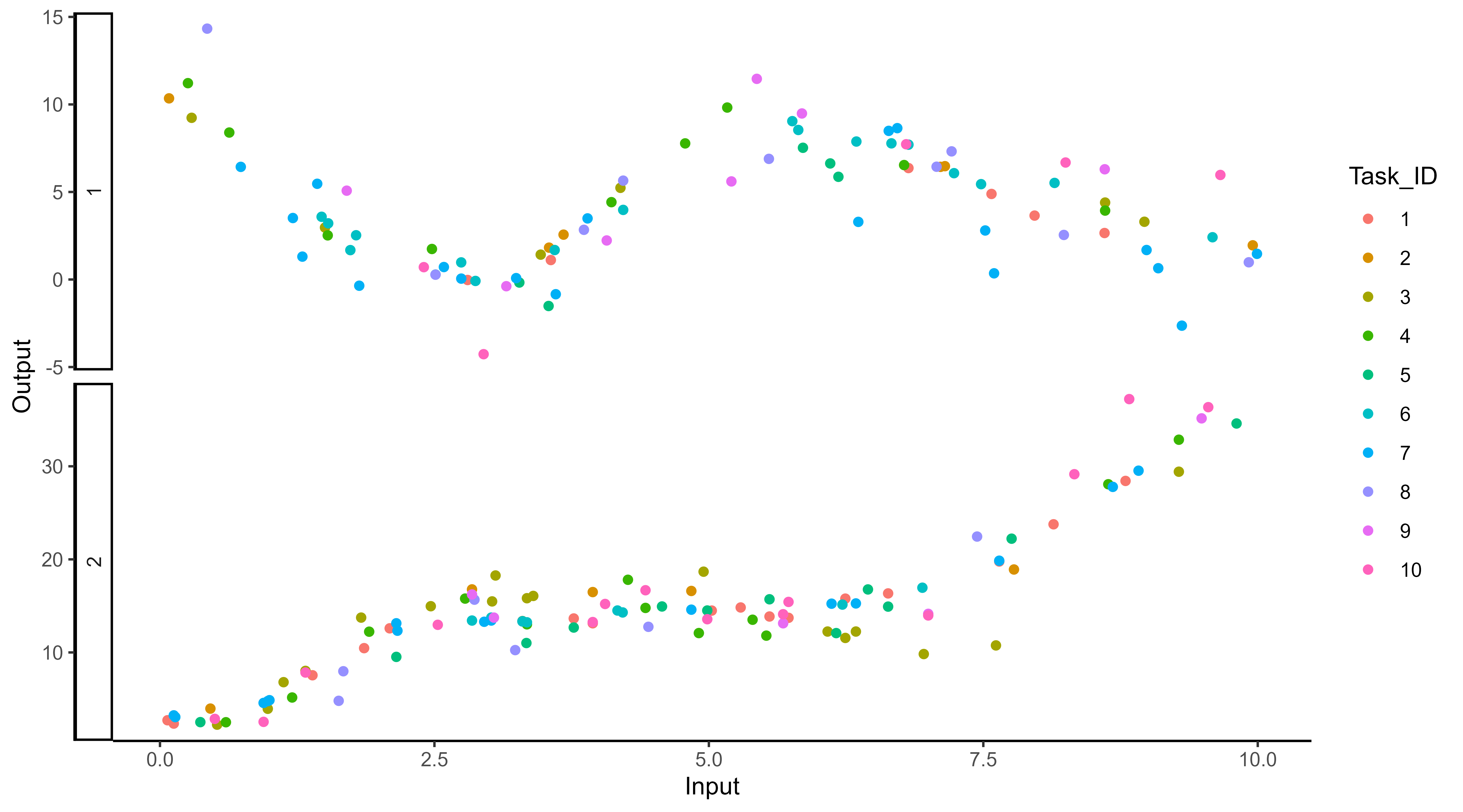
Let’s try something difficult

For instance, this context could correspond to measuring both weight and milk production of several cows over time, of unknown distinct races (that we want to recover), and for which we want to predict missing values of one Output, or forecast future values of both.

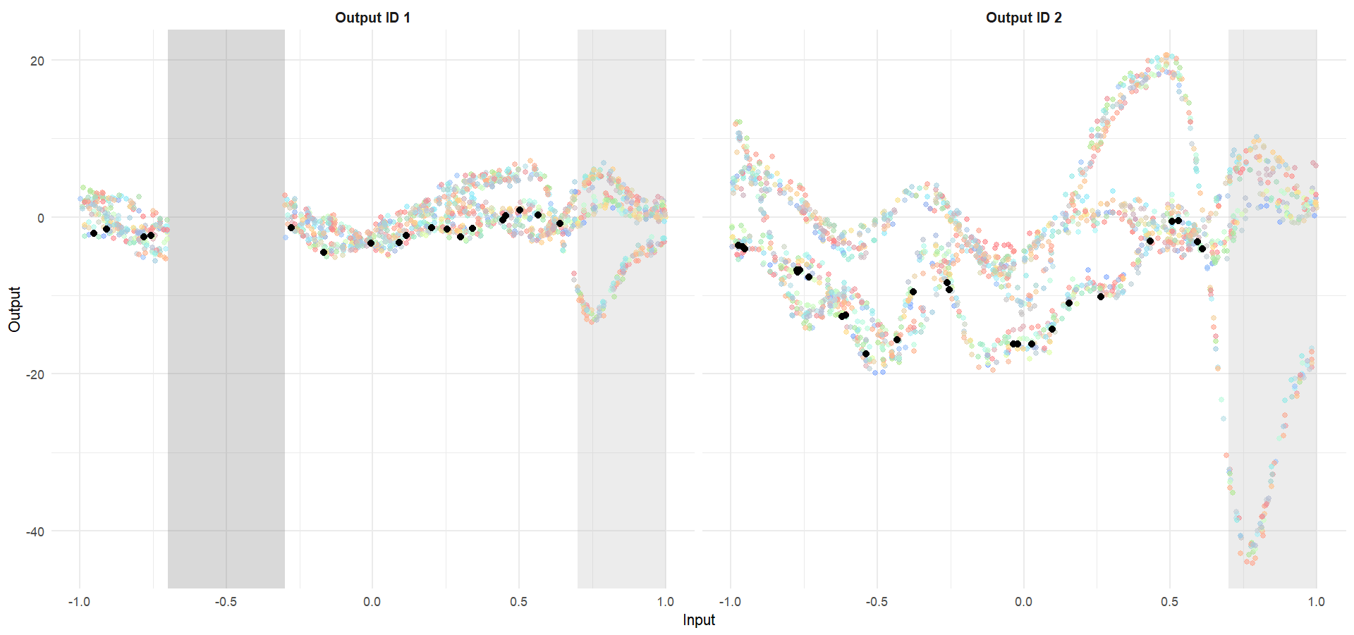
Let’s try something difficult

Let’s remove [-0.7, -0.3] of 2nd Output, and [0.7, 1] of both Outputs for the testing Task, and try to predict the those testing points (and recover the underlying clusters).

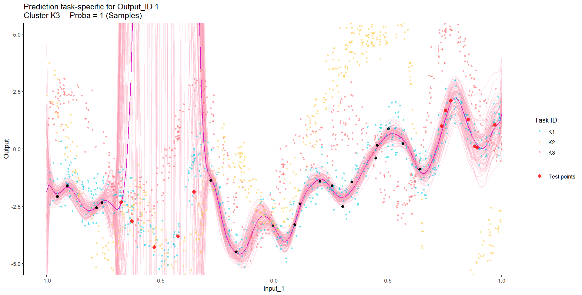
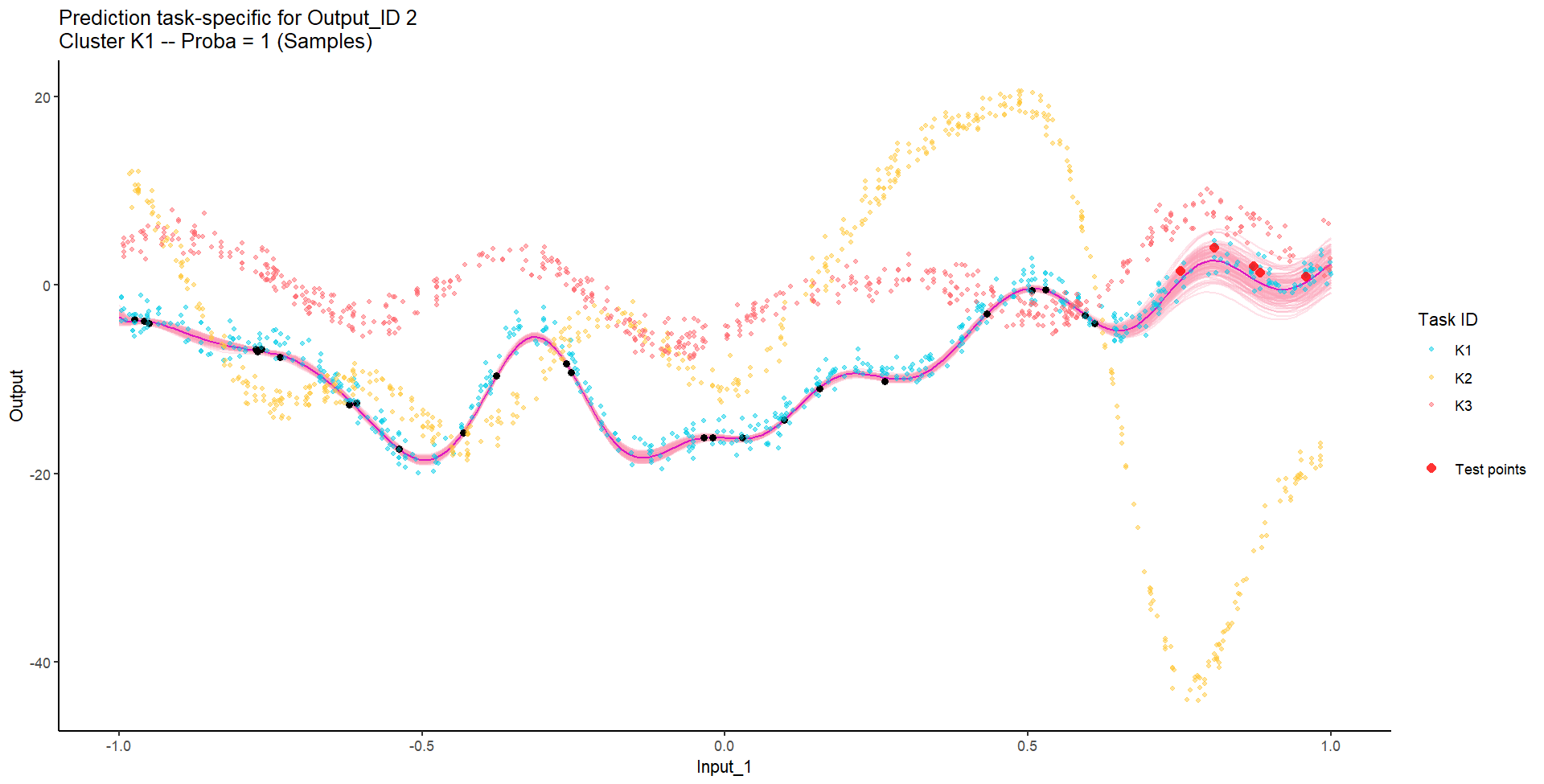
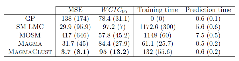
We don’t even try vanilla GPs, maybe Multi-Output GPs?

• Output 1
• Output 2

Perhaps Multi-Task GPs can do better?

• Output 1
• Output 2

Do we really get the best of both worlds?

• Output 1
• Output 2

Take home messages

• Multi-Ouput / Multi-task: the same mathematical problem can hide different intuitions on the data and lead to dedicated modelling paradigms,
• Both the mean and covariance parameters can effectively be leveraged to share information,
• Modelling jointly data coming from several sources can costs roughly the same as independant modelling, but can improve dramatically predictive capacities.

Rule of thumb:

Output nature	Framework	Complexity
Independant variables of interest	Single-Task	\(\color{red}{O}\times\mathcal{O}(N^3)\)
Correlated variables of interest	Multi-Output	\(\mathcal{O}(\color{red}{O}^3 N^3)\)
Occurences of the same phenomenon	Multi-Task	\(\mathcal{O}(\color{blue}{T} \times N^3)\)
Occurences of correlated variables	Multi-Task-Multi-Output	\(\mathcal{O}(\color{blue}{T}\times\color{red}{O}^3 N^3)\)

The crew expanding all this

We are currently working on some nice extensions with a great team of PhD students!

Alexia Grenouillat - Simon Lejoly - Térence Viellard

Some problems we are tackling (at least trying to):

• Highly efficient Python implementation (based on Jax) for MOMT GPs,
• Non-Gaussian likelihoods in the MOMT framework (adapting Laplace Matching),
• Scalability in the number of inputs, outputs, tasks, input dimensions,
• Hopefully many other problems that we’ll be happy to discuss with you in the next years

Thank you for your attention!

How about Multi-Multi-[…]-Task GPs?

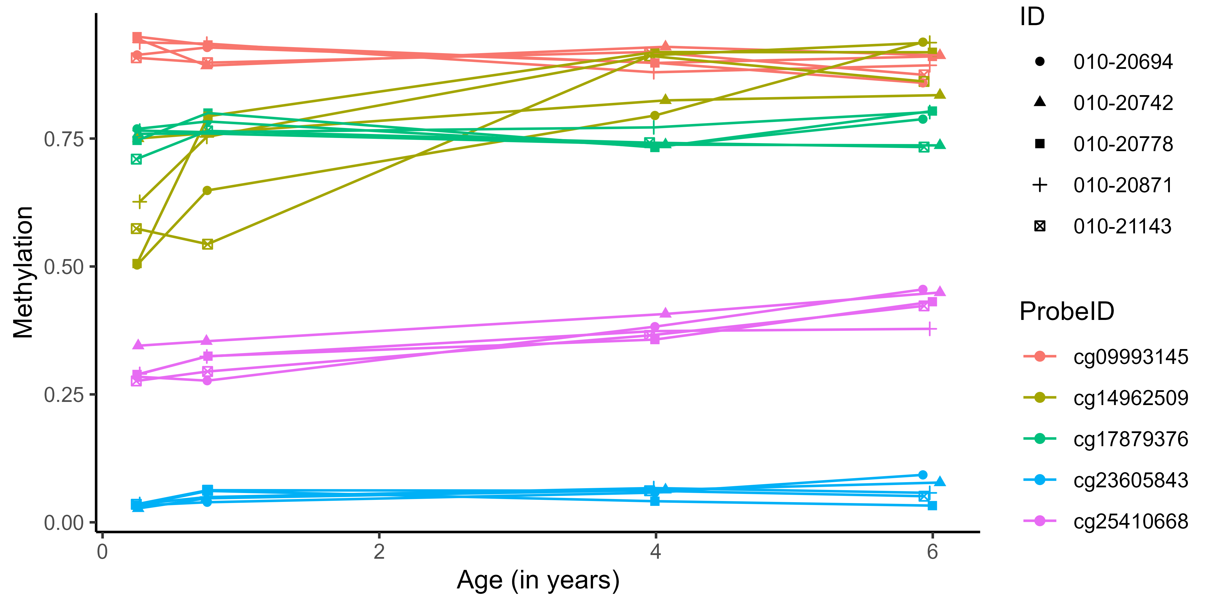
Several sources of correlation might exist in a dataset (e.g. multiple genes and individuals)

Multi-Mean Gaussian processes

\[y_{\color{blue}{i}\color{red}{j}} = \mu_{0} + f_\color{blue}{i} + g_\color{red}{j} + \epsilon_{\color{blue}{i}\color{red}{j}}\]

with:

• \(\mu_{0} \sim \mathcal{GP}(m_{0}, {C_{\gamma_{0}}}), \ f_{\color{blue}{i}} \sim \mathcal{GP}(0, \Sigma_{\theta_{\color{blue}{i}}}), \ \epsilon_{\color{blue}{i}\color{red}{j}} \sim \mathcal{GP}(0, \sigma_{\color{blue}{i}\color{red}{j}}^2), \ \perp \!\!\! \perp_t\)
• \(g_{\color{red}{j}} \sim \mathcal{GP}(0, \Sigma_{\theta_{\color{red}{j}}})\)

Key idea for training: define \(\color{blue}{T}+\color{red}{P} + 1\) different hyper-posterior distributions for \(\mu_0\) by conditioning over the adequate sub-sample of data.

\[p(\mu_0 \mid \{y_{\color{blue}{i}\color{red}{j}} \}_{\color{red}{j} = 1,\dots, \color{red}{P}}^{\color{blue}{i} = 1,\dots, \color{blue}{T}}) = \mathcal{N}\Big(\mu_{0}; \ \hat{m}_{0}, \hat{K}_0 \Big).\]

\[p(\mu_0 \mid \{y_{\color{blue}{i}\color{red}{j}} \}_{\color{blue}{i} = 1,\dots, \color{blue}{T}}) = \mathcal{N}\Big(\mu_{0}; \ \hat{m}_{\color{red}{j}}, \hat{K}_\color{red}{j} \Big), \ \forall \color{red}{j} \in 1, \dots, \color{red}{P}\]

\[p(\mu_0 \mid \{y_{\color{blue}{i}\color{red}{j}} \}_{\color{red}{j} = 1,\dots, \color{red}{P}}) = \mathcal{N}\Big(\mu_{0}; \ \hat{m}_{\color{blue}{i}}, \hat{K}_\color{blue}{i} \Big), \forall \color{blue}{i} \in 1, \dots, \color{blue}{T} \]

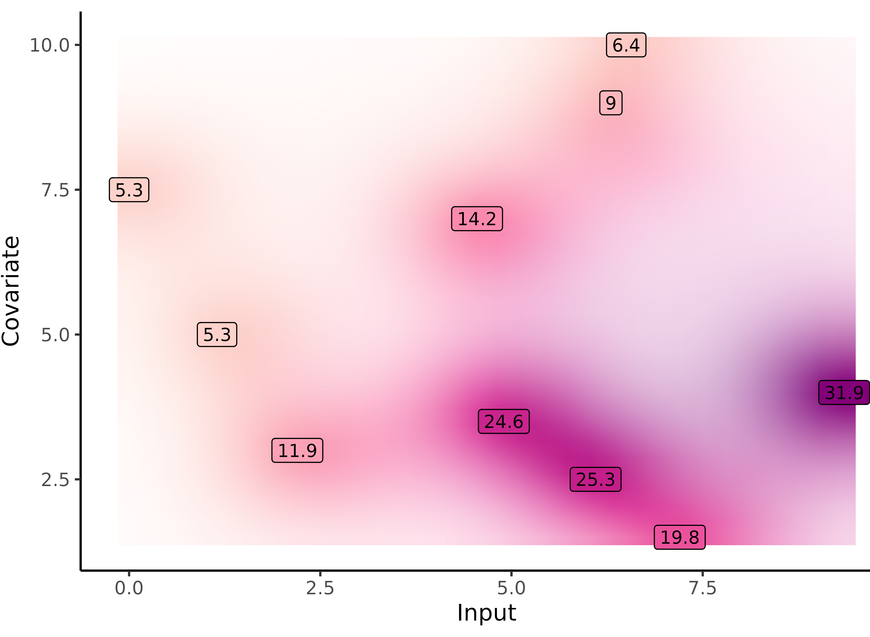
Multi-Mean GPs: multiple hyper-posterior mean processes

Each sub-sample of data leads to a specific hyper-posterior distribution of the mean process \(\mu_0\).

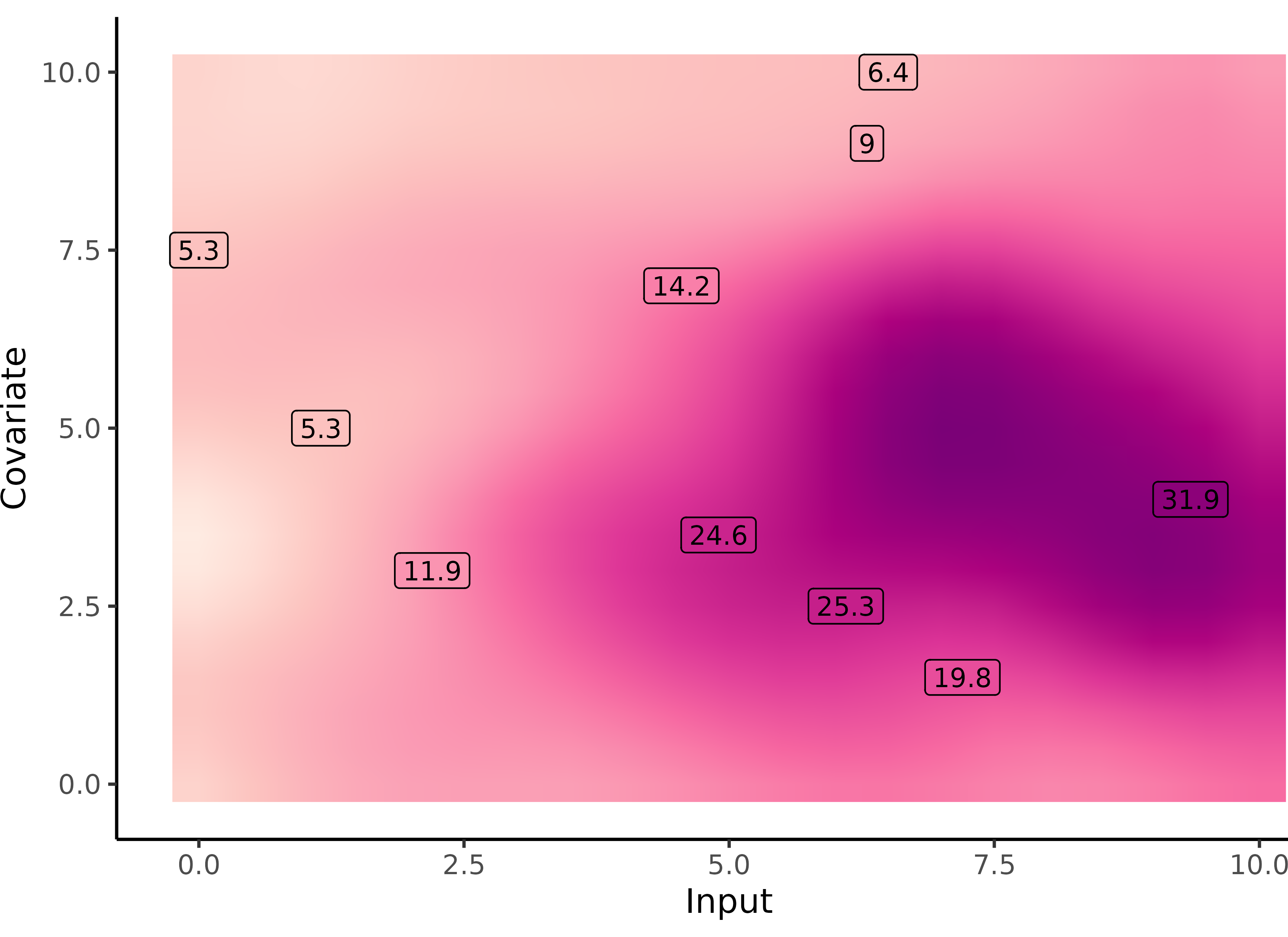
Multi-Mean GPs: an adaptive prediction

Although sharing the same mean process, different tasks still lead to different predictions.

Multi-mean GP provides adaptive predictions according to the relevant context.

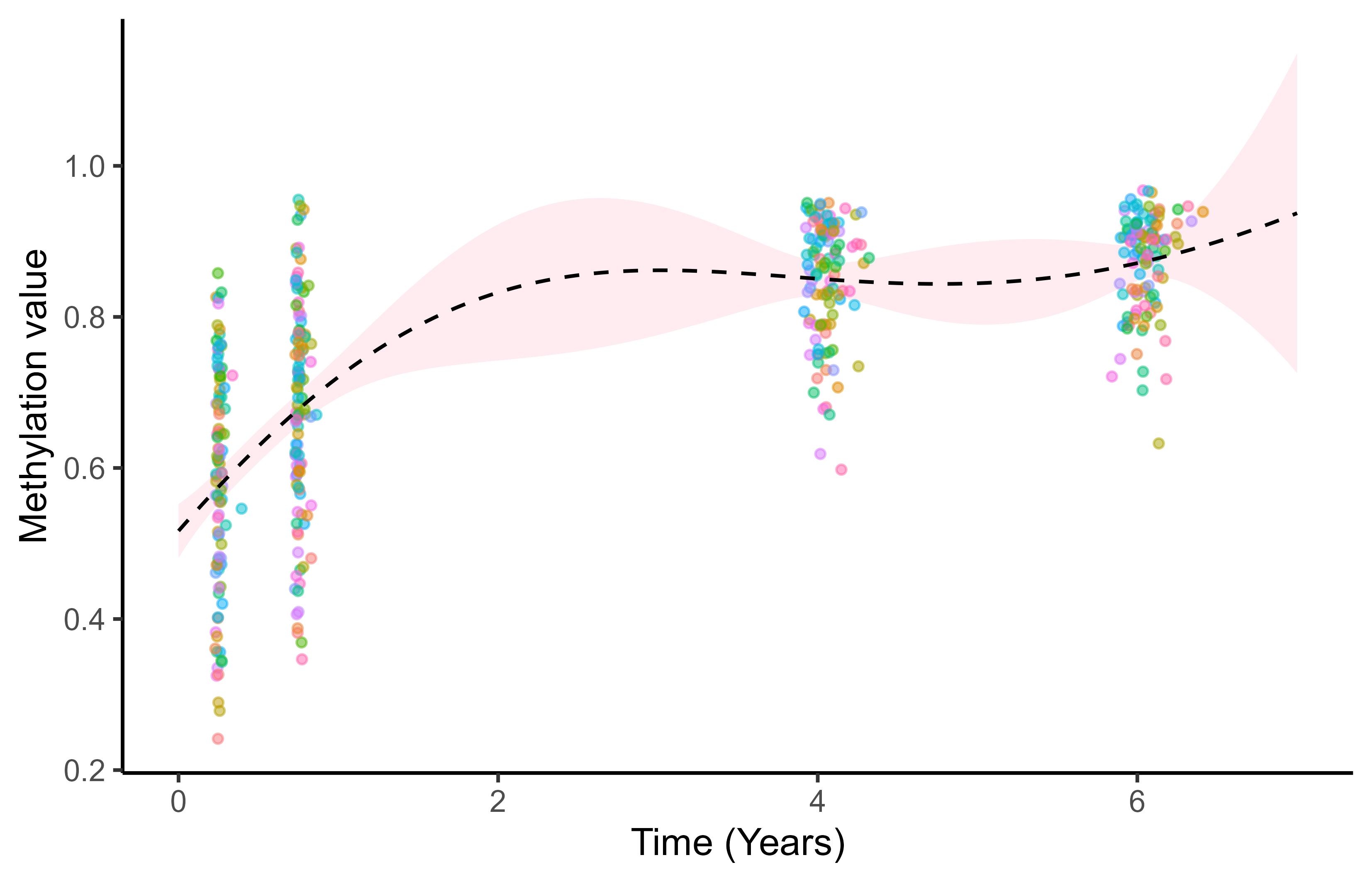
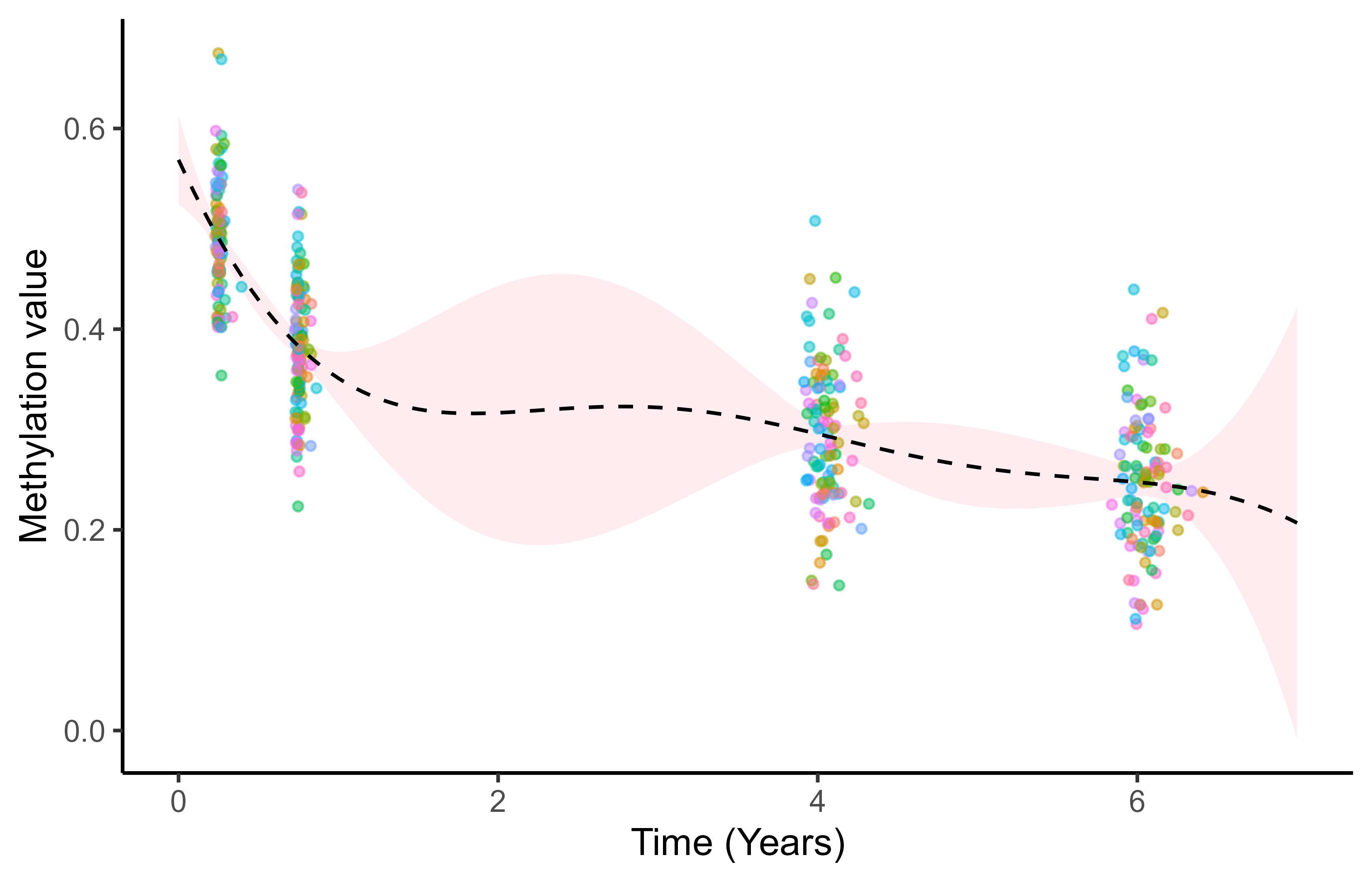
Forecasting thousands of genenomic time series…

… with the adequate quantification of uncertainty

Performance of MagmaClust

Model selection performances of VBIC