---

Functional Data,
Multi-Output and Multi-Task
Gaussian Processes

---

Arthur Leroy - GABI & MIA Paris Saclay, INRAE

Withings meeting - 14/11/2025

Can you spot the difference?

Can you spot the difference?

Functional data is all about smoothness and tidiness

Functional data is all about smoothness and tidiness

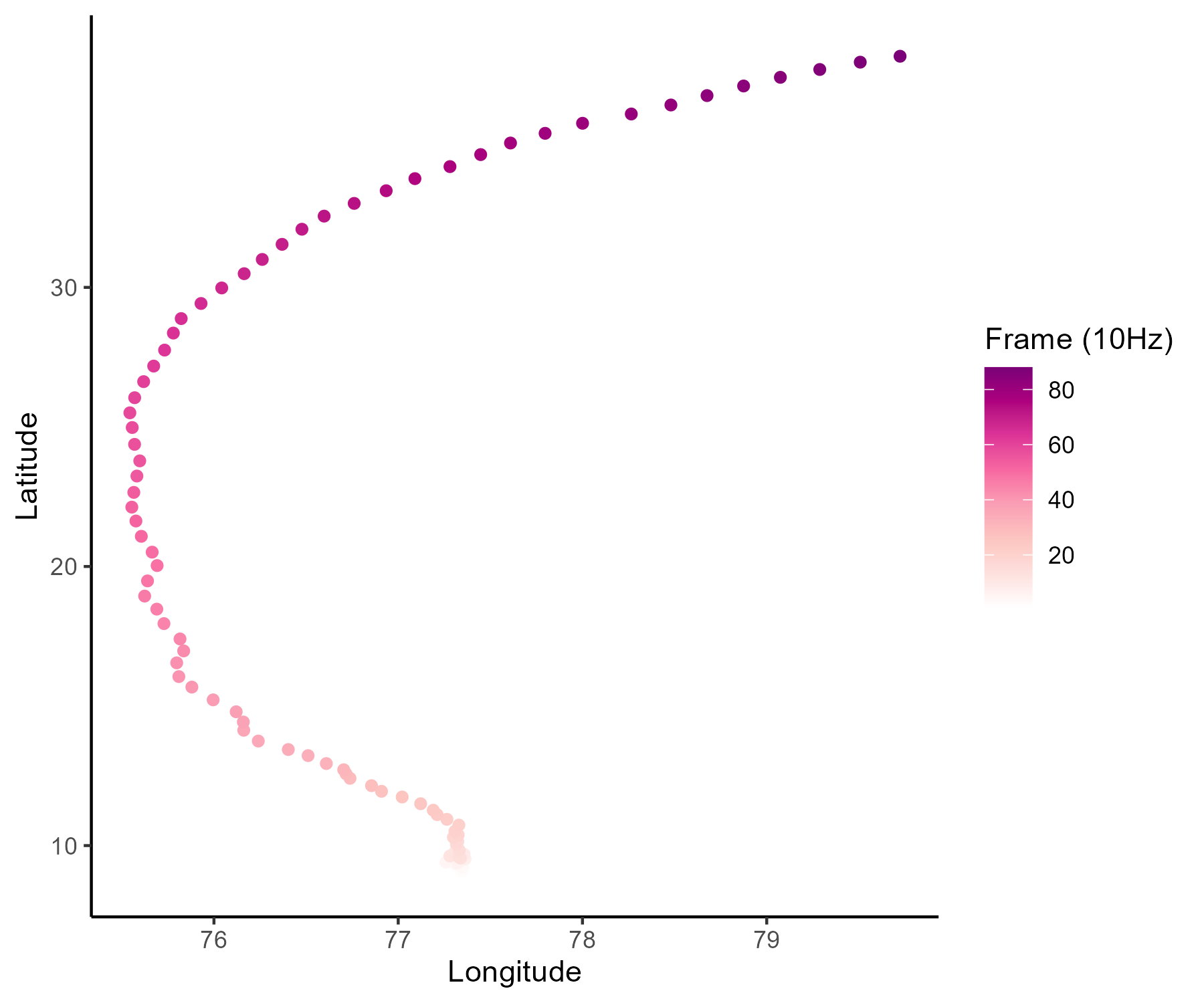
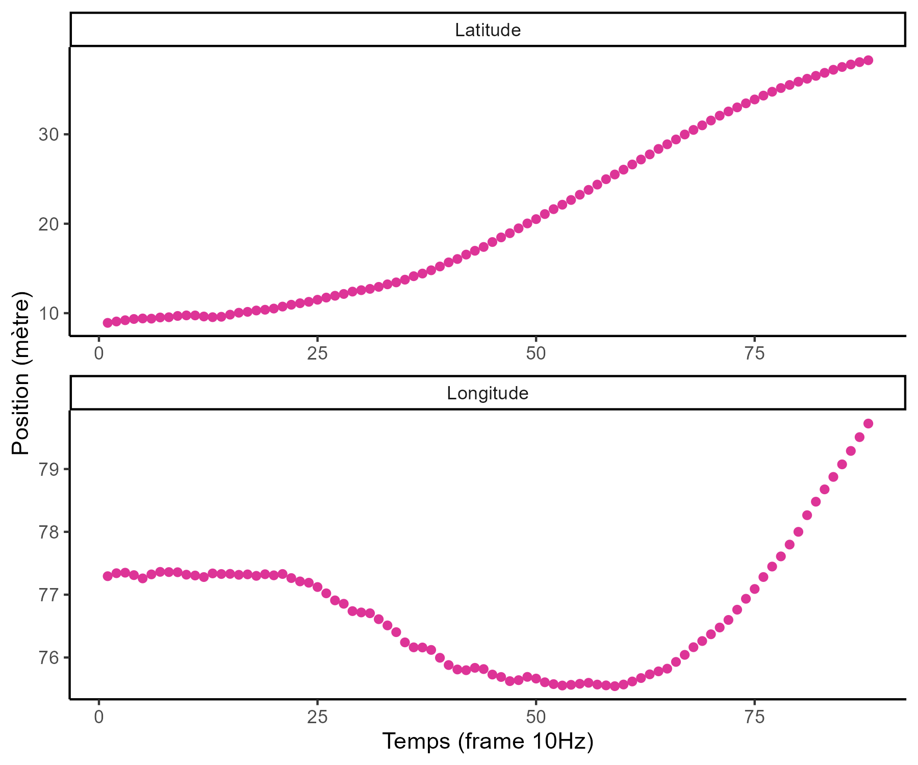
Functional data in real-life problems ? Time, space and continua

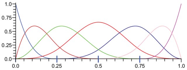
Reconstructing functions from series of points

A function can be expressed as a linear combination of basis functions: \[f(t) = \sum\limits_{b=1}^{B}{\alpha_b \ \phi_b(t)}\]

If we observed the function at \(N\) instants, we can find coefficients \(\boldsymbol{\alpha}\) through least squares:

\[LS(\boldsymbol{\alpha}) = \sum_{i=1}^{N}\left[f(t_i)-\sum_{b = 1}^{B} \alpha_{b} \phi_{b}\left(t_{i}\right)\right]^{2}\]

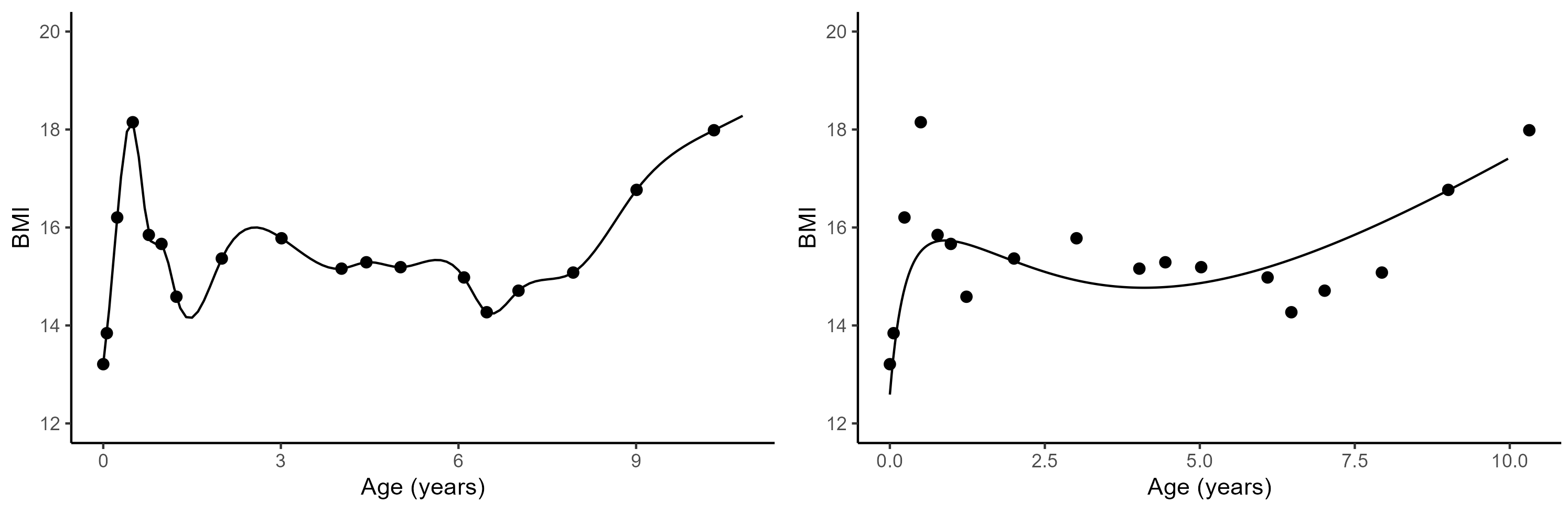
Functional data analysis is the art of drawing curves from points

Depending on the context, we may expect different properties for our function.

Do we interpolate or smooth? Are the variations periodic (Fourier basis), multi-scale (wavelets) or polynomial (B-splines)? Answers are probably is this book.

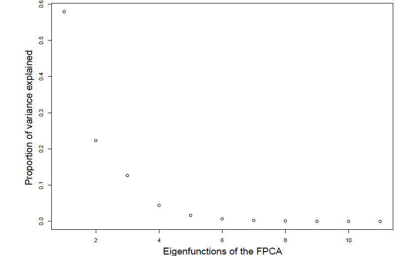
Functional Principal Component Analysis (FPCA)

Like for multi-variate statistics, FCPA is central method when studying functions. From the Karhunen-Loève theorem we can express any centred stochastic process as an infinite linear combination of orthonormal eigenfunctions:

\[X(t)-\mathbb{E}[X(t)]=\sum_{q=1}^{\infty} \xi_{q} \varphi_{q}(t)\]

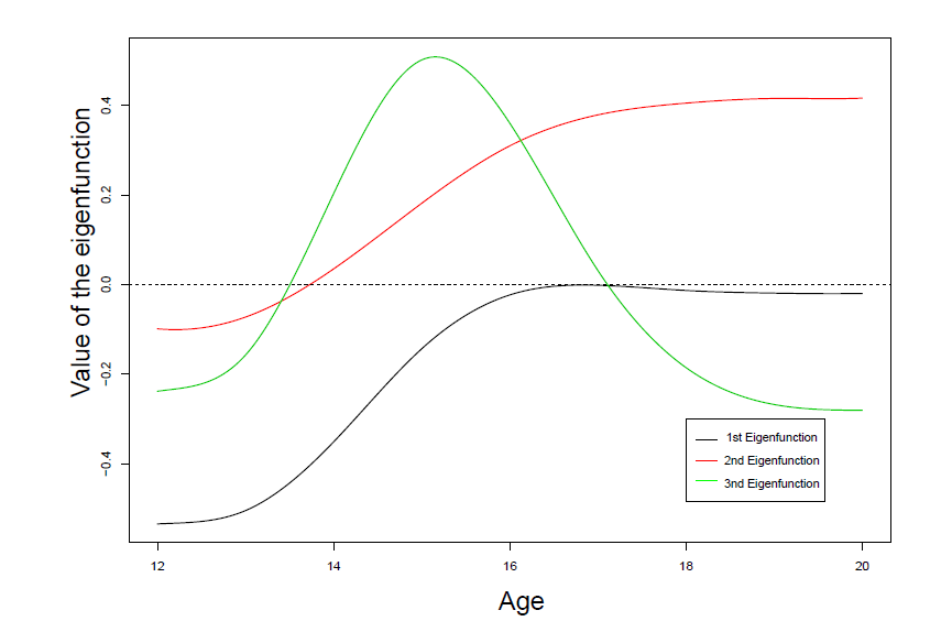
I must admit, it’s a bit trickier to interpret

It’s still used to represent the trajectories explaining the most variance among our functions. Eigenfunctions are uncorrelated, and they provide the most parsimonious decomposition in terms of basis function.

The curse of dimensionality? Don’t care, I’m smooth

One nice and surprising property of FDA methods is that they generally don’t suffer from being infinitely high dimensional. Intuitively, what is the true dimension of this object?

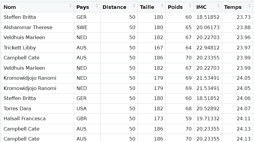
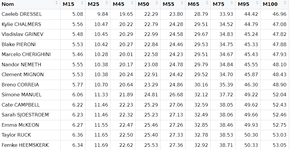
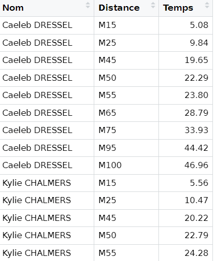
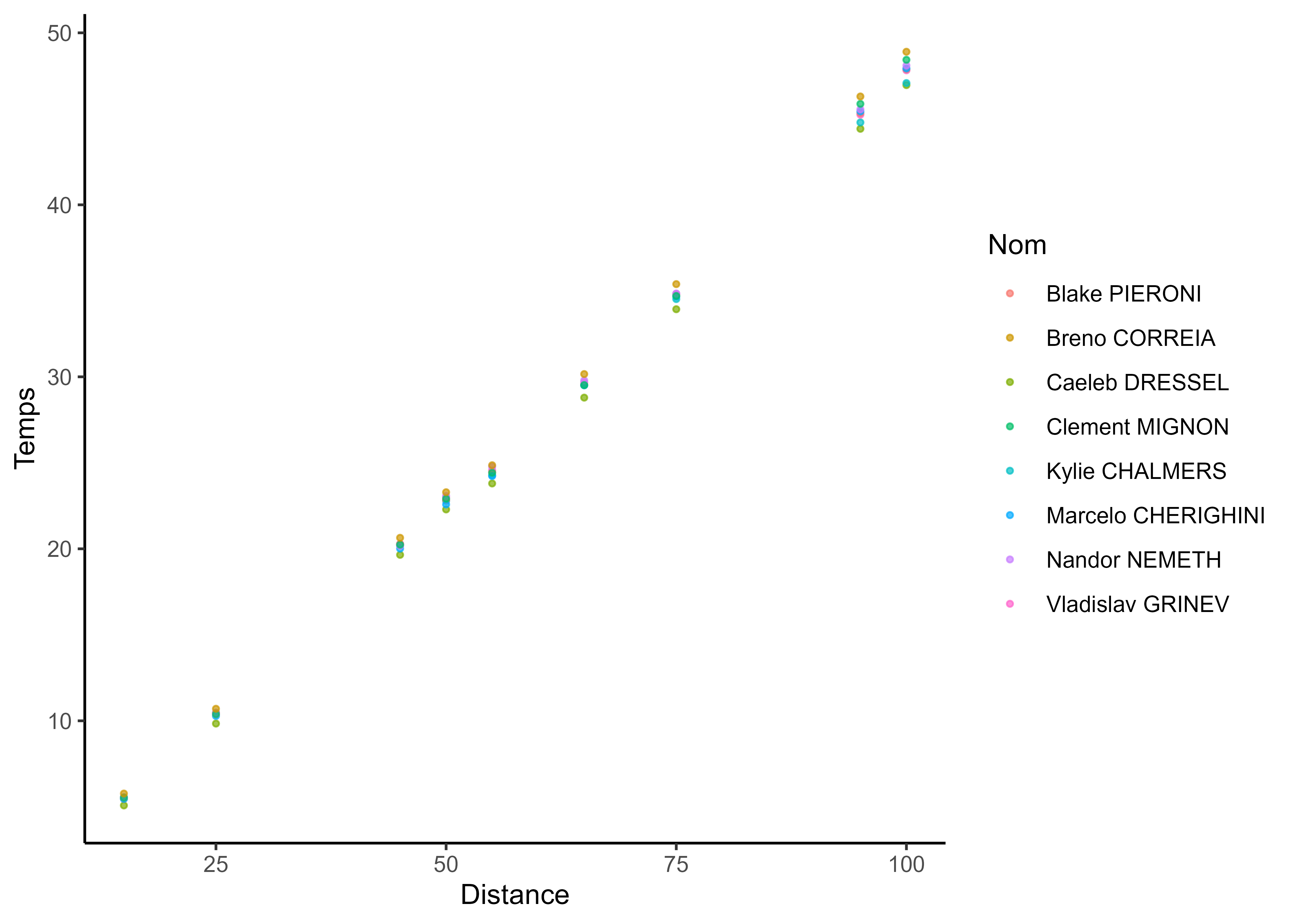
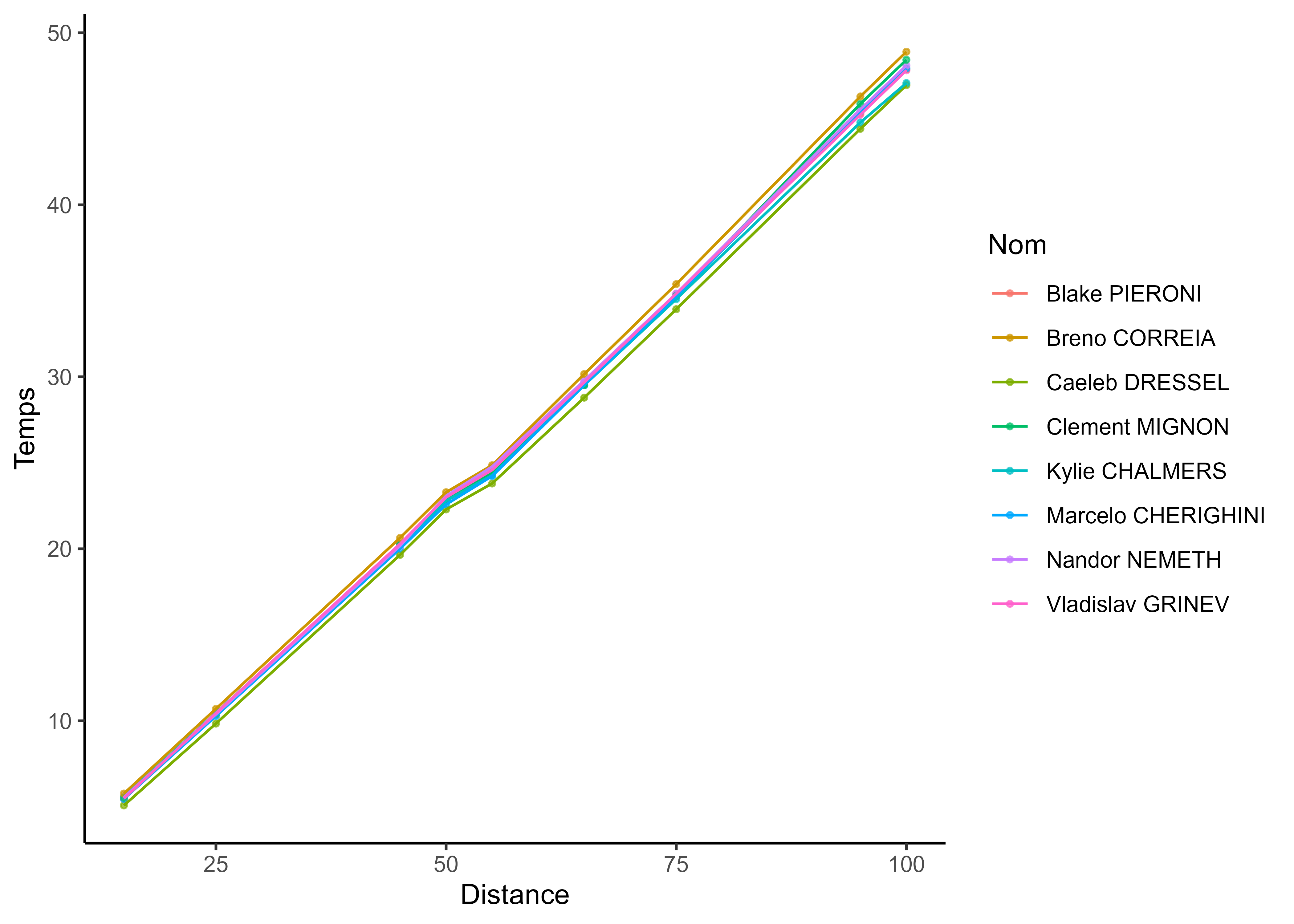
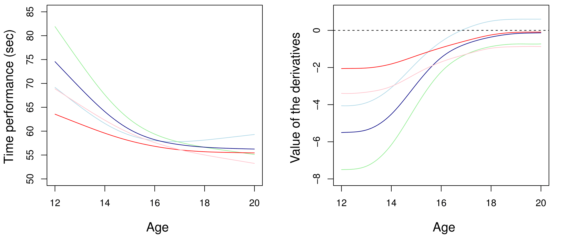
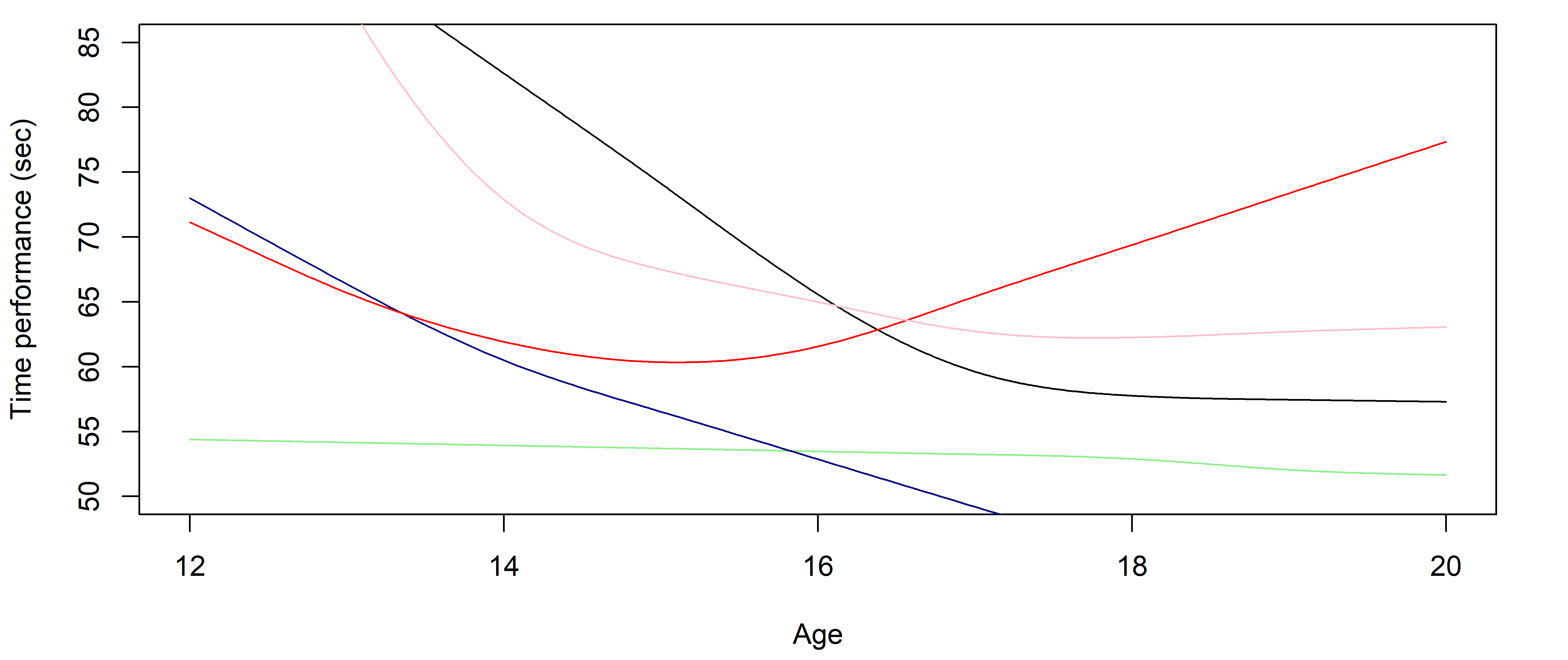
Modelling functions gives you derivatives to study dynamics

Clustering performance curves of 100m freestyle swimmers into 5 groups using derivatives.

FDA is limited (and it’s kinda old to be fair)

• While average trajectories of groups are reasonable, individual curves may easily diverge,
• Really low predictive capacities,
• No quantification of uncertainty.

Probabilistic modelling and predictions: how do we really learn?

Moving from exploring to learning functions

\[y = \color{orange}{f}(x) + \epsilon\]

where:

• \(x\) is the input variable (typically time, location, any continuum),
• \(y\) is the output variable (any measurement of interest),
• \(\epsilon\) is the noise, a random error term,
• \(\color{orange}{f}\) is a random function encoding the relationship between input and output data.

All supervised learning problems require to retrieve the most reliable function \(\color{orange}{f}\), using observed data \(\{(x_1, y_1), \dots, (x_n, y_n) \}\), to perform predictions when observing new input data \(x_{n+1}\).

Learning the simplest of functions : linear regression

In the simplest (though really common in practice) case of linear regression, we assume that:

\[\color{orange}{f}(x) = a x + b\]

Finding the best function \(\color{orange}{f}\) reduces to compute optimal parameters \(a\) and \(b\) from our dataset.

Learning is about updating our knowledge

This well-known probability formula has massive implications on learning strategies:

\[\mathbb{P}(\color{red}{T} \mid \color{blue}{D}) = \dfrac{\mathbb{P}(\color{blue}{D} \mid \color{red}{T}) \times \mathbb{P}(\color{red}{T})}{\mathbb{P}(\color{blue}{D})}\]

with:

• \(\mathbb{P}(\color{red}{T})\), probability that some theory \(\color{red}{T}\) is true, our prior belief.
• \(\mathbb{P}(\color{blue}{D} \mid \color{red}{T})\), probability to observe this data if theory \(\color{red}{T}\) is true, the likelihood.
• \(\mathbb{P}(\color{blue}{D})\), probability to observe this data overall, often called the evidence.

Bayes’ theorem indicates how to update our beliefs about \(\color{red}{T}\) when accounting for new data \(\color{blue}{D}\) :

• \(\mathbb{P}(\color{red}{T} \mid \color{blue}{D})\), probability that theory \(\color{red}{T}\) is true considering data \(\color{blue}{D}\), our posterior belief.

A visual explanation of Bayes’ theorem

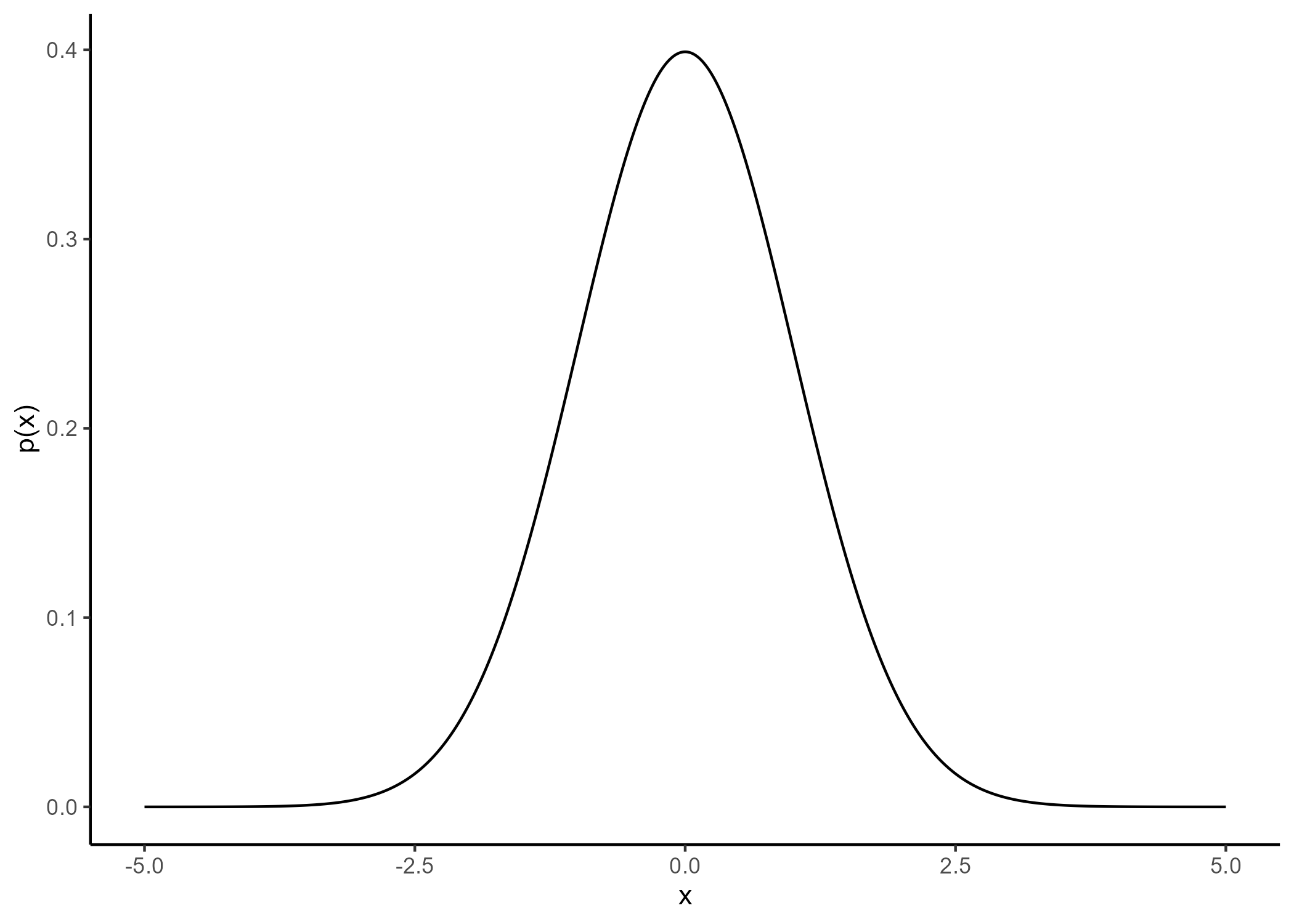
We generally use probability distributions to express our initial uncertainty about a quantity of interest (balance of a coin, average size of a human, …) and its posterior probable values.

Probabilistic estimation can be an alternative to testing

Let’s exercise your Bayesian mind

Assume there exists some trouble or disease such that:

• \(\mathbb{P}(\color{red}{T}) = 0.001,\) 1 person out of 1000 contracted the trouble on average,
• \(\mathbb{P}(\color{blue}{D} \mid \color{red}{T}) = 0.99,\) a detection test is 99% reliable if you have the trouble,
• \(\mathbb{P}(\color{blue}{\bar{D}} \mid \color{red}{\bar{T}}) = 0.99,\) this same detection test is 99% reliable if you don’t have the trouble,

From Bayes’ theorem, the probability to have contracted the trouble when the detection test was positive is:

\[\mathbb{P}(\color{red}{T} \mid \color{blue}{D}) = \dfrac{\mathbb{P}(\color{blue}{D} \mid \color{red}{T}) \times \mathbb{P}(\color{red}{T})}{\mathbb{P}(\color{blue}{D})} = \dfrac{0.99 \times 0.001}{0.99 \times 0.001 + (1-0.99) \times 0.999} \simeq 0.09\]

Hence, we only have 9% chance to actually be sick despite a positive result to the detection test.

Gaussian process: a prior distribution over functions

\[y = \color{orange}{f}(x) + \epsilon\]

No restrictions on \(\color{orange}{f}\) but a prior distribution on a functional space: \(\color{orange}{f} \sim \mathcal{GP}(m(\cdot),C(\cdot,\cdot))\)

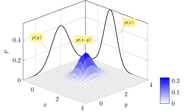
We can think of a Gaussian process as the extension to infinity of multivariate Gaussians:
      \(x \sim \mathcal{N}(m , \sigma^2)\) in \(\mathbb{R}\),       \(\begin{pmatrix} x_1 \\ x_2 \\ \end{pmatrix} \sim \mathcal{N} \left( \ \begin{pmatrix} m_1 \\ m_2 \\ \end{pmatrix}, \begin{bmatrix} C_{1,1} & C_{1,2} \\ C_{2,1} & C_{2,2} \end{bmatrix} \right)\) in \(\mathbb{R}^2\)

     
Credits: Raghavendra Selvan

A GP is like a long cake and each slice is a Gaussian

Credits: Carl Henrik Ek

A GP is like an infinitely long cake and each slice is a Gaussian

Credits: Carl Henrik Ek

Covariance functions: Squared Exponential kernel

While \(m(\cdot)\) is often assumed to be \(0\), the covariance structure is critical and defined through tailored kernels. For instance, the Squared Exponential (or RBF) kernel is expressed as: \[C_{SE}(x, x^{\prime}) = s^2 \exp \Bigg(-\dfrac{(x - x^{\prime})^2}{2 \ell^2}\Bigg)\]

Covariance functions: Periodic kernel

To model phenomenon exhibiting repeting patterns, one can leverage the Periodic kernel: \[C_{perio}(x, x^{\prime}) = s^2 \exp \Bigg(- \dfrac{ 2 \sin^2 \Big(\pi \frac{\mid x - x^{\prime}\mid}{p} \Big)}{\ell^2}\Bigg)\]

Covariance functions: Linear kernel

We can even consider linear regression as a particular GP problem, by using the Linear kernel: \[C_{lin}(x, x^{\prime}) = s_a^2 + s_b^2 (x - c)(x^{\prime} - c )\]

We can learn optimal values of hyper-parameters from data through maximum likelihood.

Gaussian process: all you need is a posterior

The Gaussian property induces that unobserved points have no influence on inference:

\[ \int \underbrace{p(f_{\color{grey}{obs}}, f_{\color{purple}{mis}})}_{\mathcal{GP}(m, C)} \ \mathrm{d}f_{\color{purple}{mis}} = \underbrace{p(f_{\color{grey}{obs}})}_{\mathcal{N}(m_{\color{grey}{obs}}, C_{\color{grey}{obs}})} \]

This crucial trick allows us to learn function properties from finite sets of observations. More generally, Gaussian processes are closed under conditioning and marginalisation.

\[ \begin{bmatrix} f_{\color{grey}{o}} \\ f_{\color{purple}{m}} \\ \end{bmatrix} \sim \mathcal{N} \left( \begin{bmatrix} m_{\color{grey}{o}} \\ m_{\color{purple}{m}} \\ \end{bmatrix}, \begin{pmatrix} C_{\color{grey}{o, o}} & C_{\color{grey}{o}, \color{purple}{m}} \\ C_{\color{purple}{m}, \color{grey}{o}} & C_{\color{purple}{m, m}} \end{pmatrix} \right) \]

While marginalisation serves for training, conditioning leads the key GP prediction formula:

\[f_{\color{purple}{m}} \mid f_{\color{grey}{o}} \sim \mathcal{N} \Big( m_{\color{purple}{m}} + C_{\color{purple}{m}, \color{grey}{o}} C_{\color{grey}{o, o}}^{-1} (f_{\color{grey}{o}} - m_{\color{grey}{o}}), \ \ C_{\color{purple}{m, m}} - C_{\color{purple}{m}, \color{grey}{o}} C_{\color{grey}{o, o}}^{-1} C_{\color{grey}{o}, \color{purple}{m}} \Big)\]

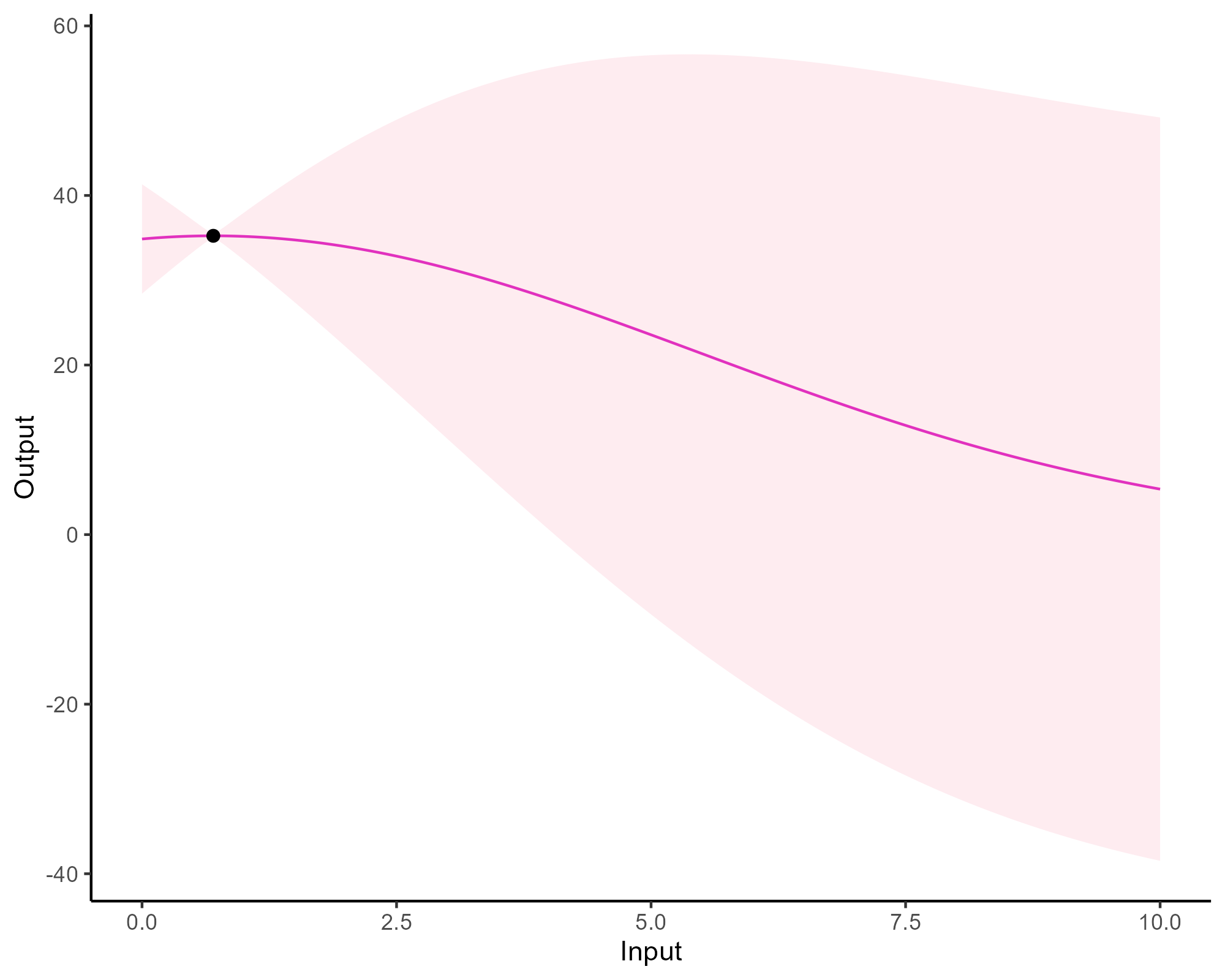
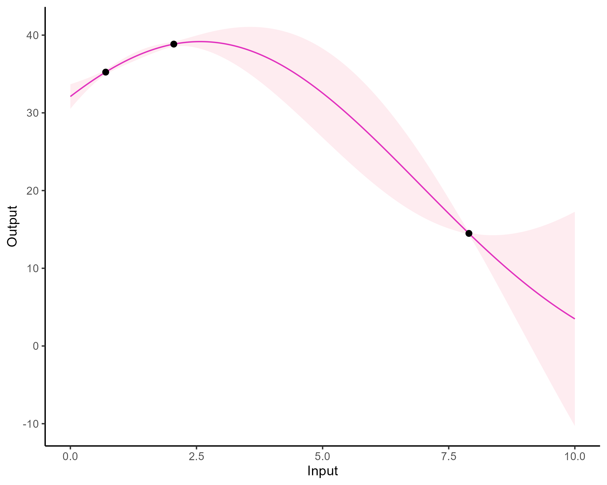
A visual explanation of GP regression

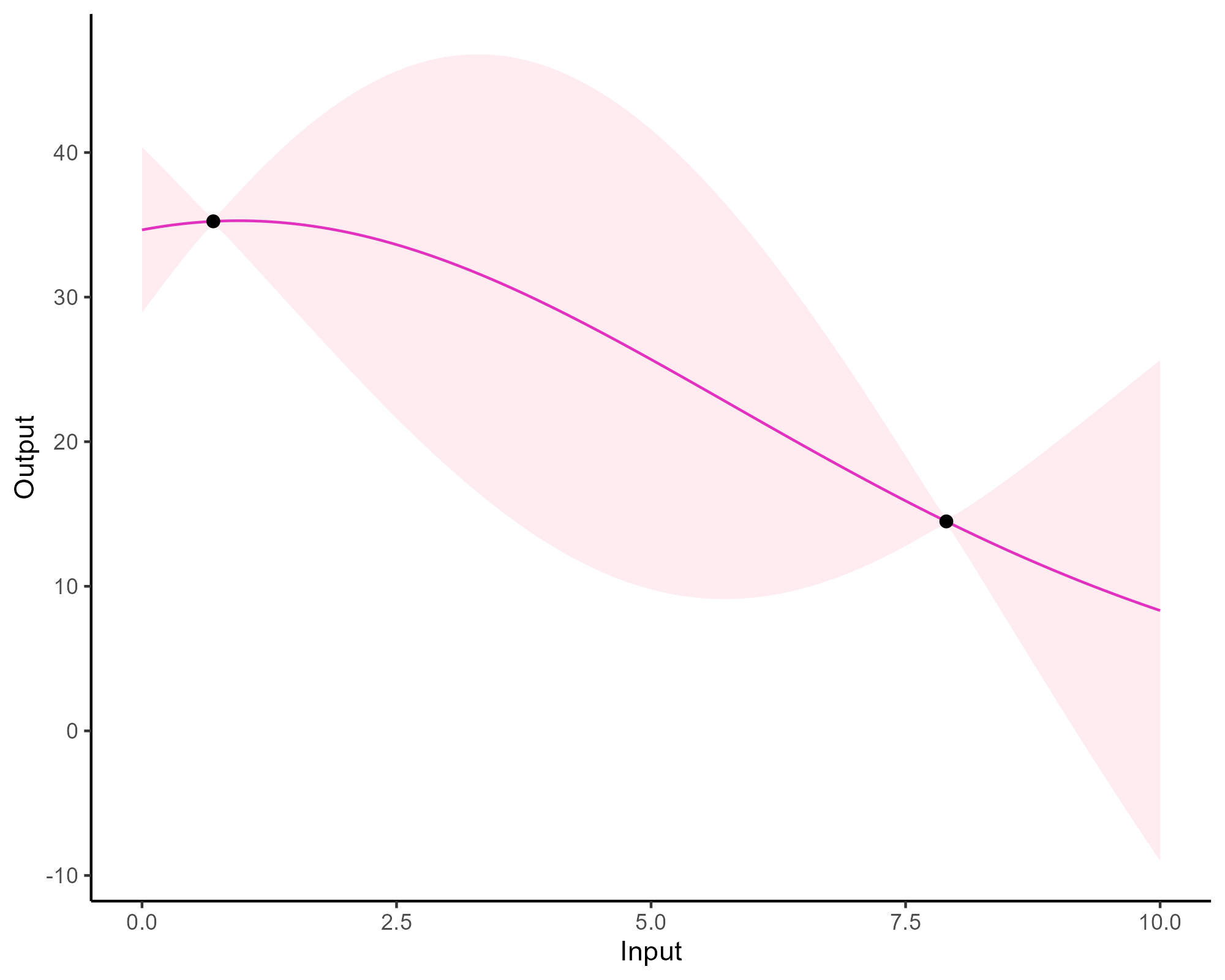
Updating our knowledge about functions

Updating our knowledge about functions

Updating our knowledge about functions

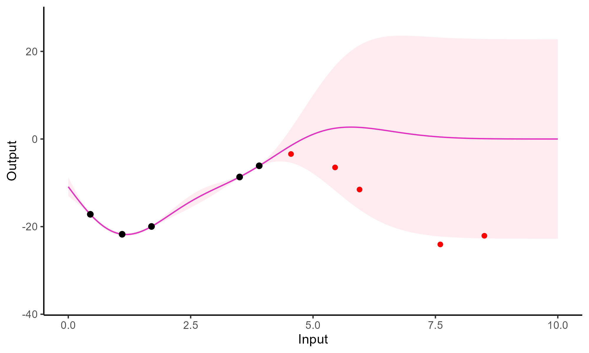
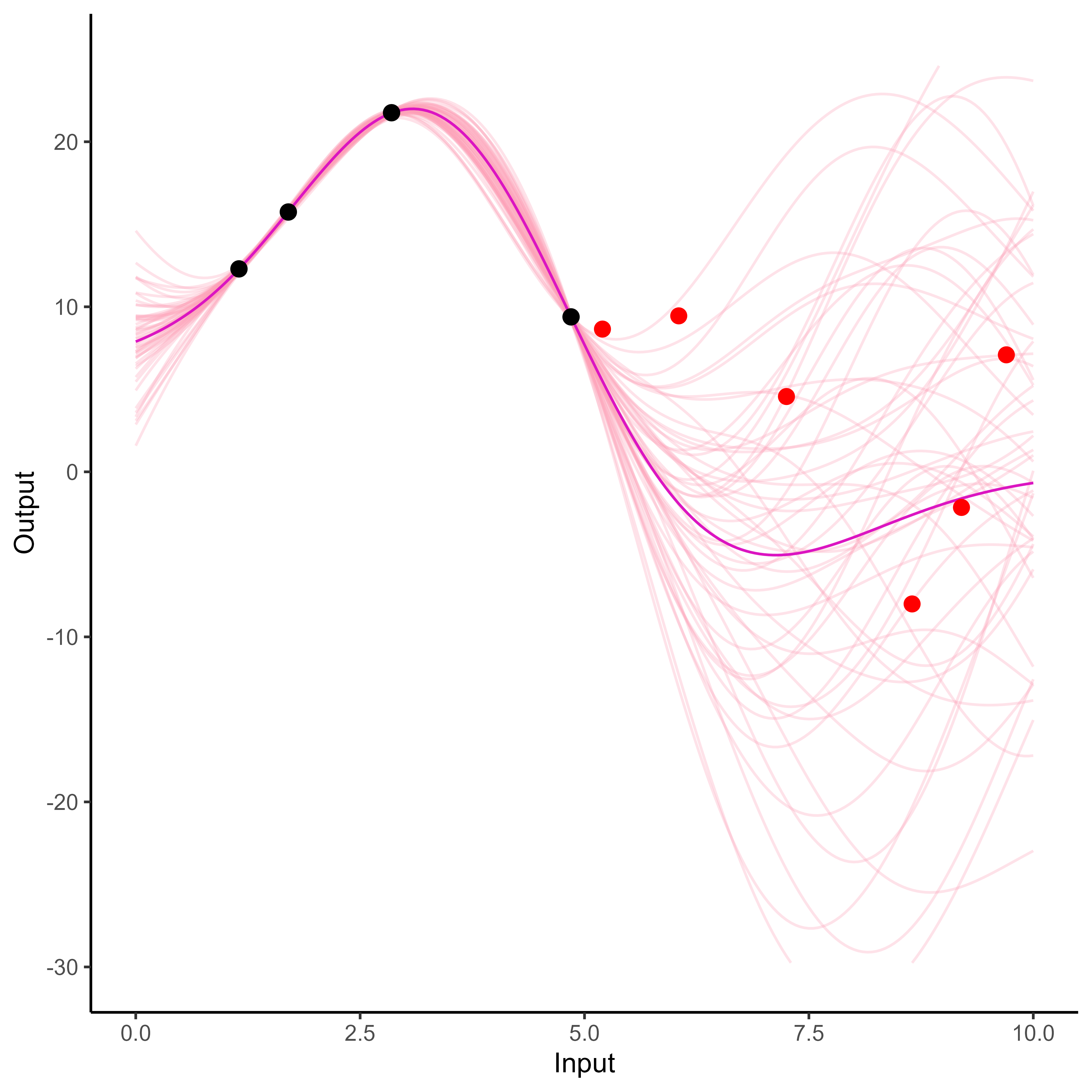
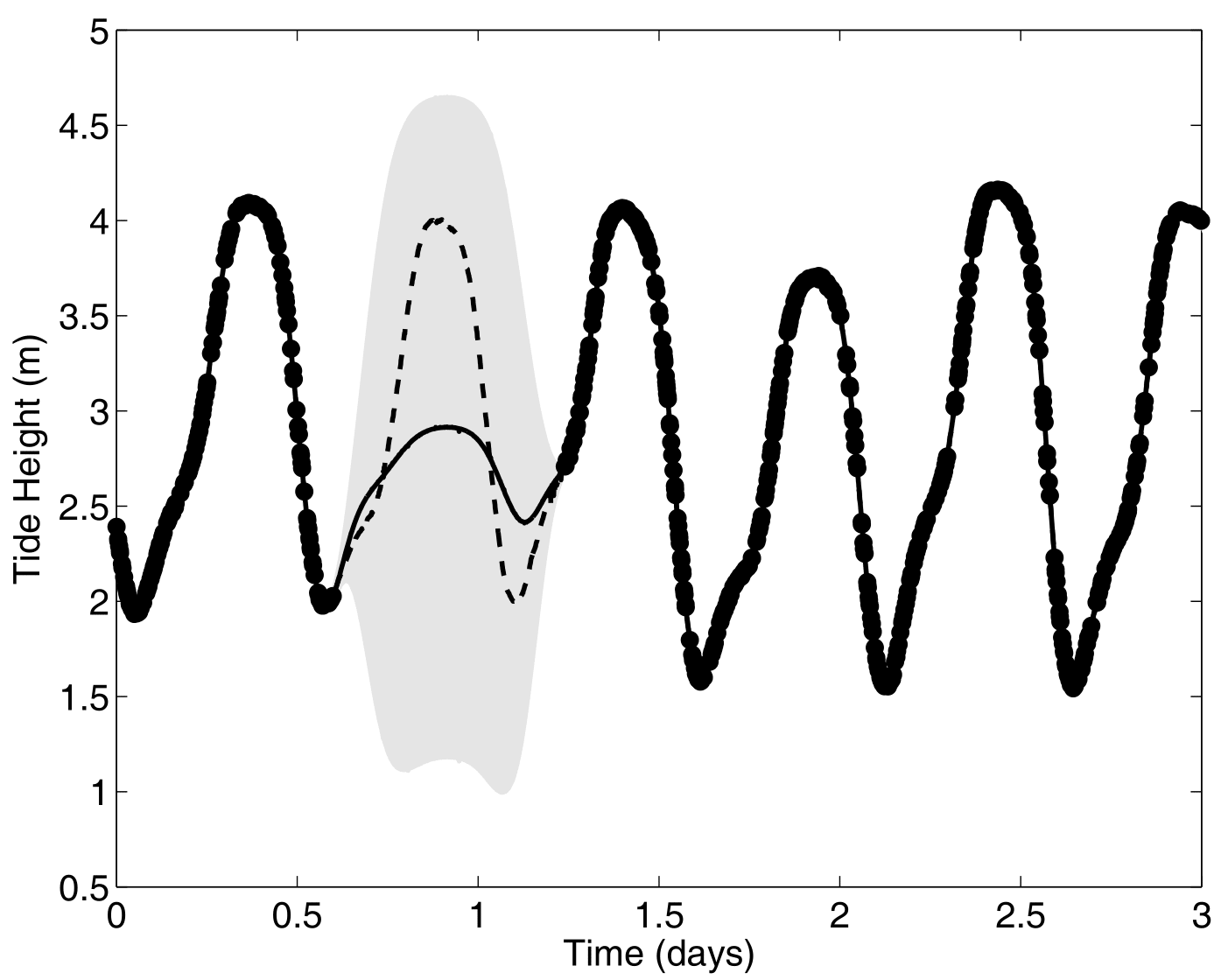
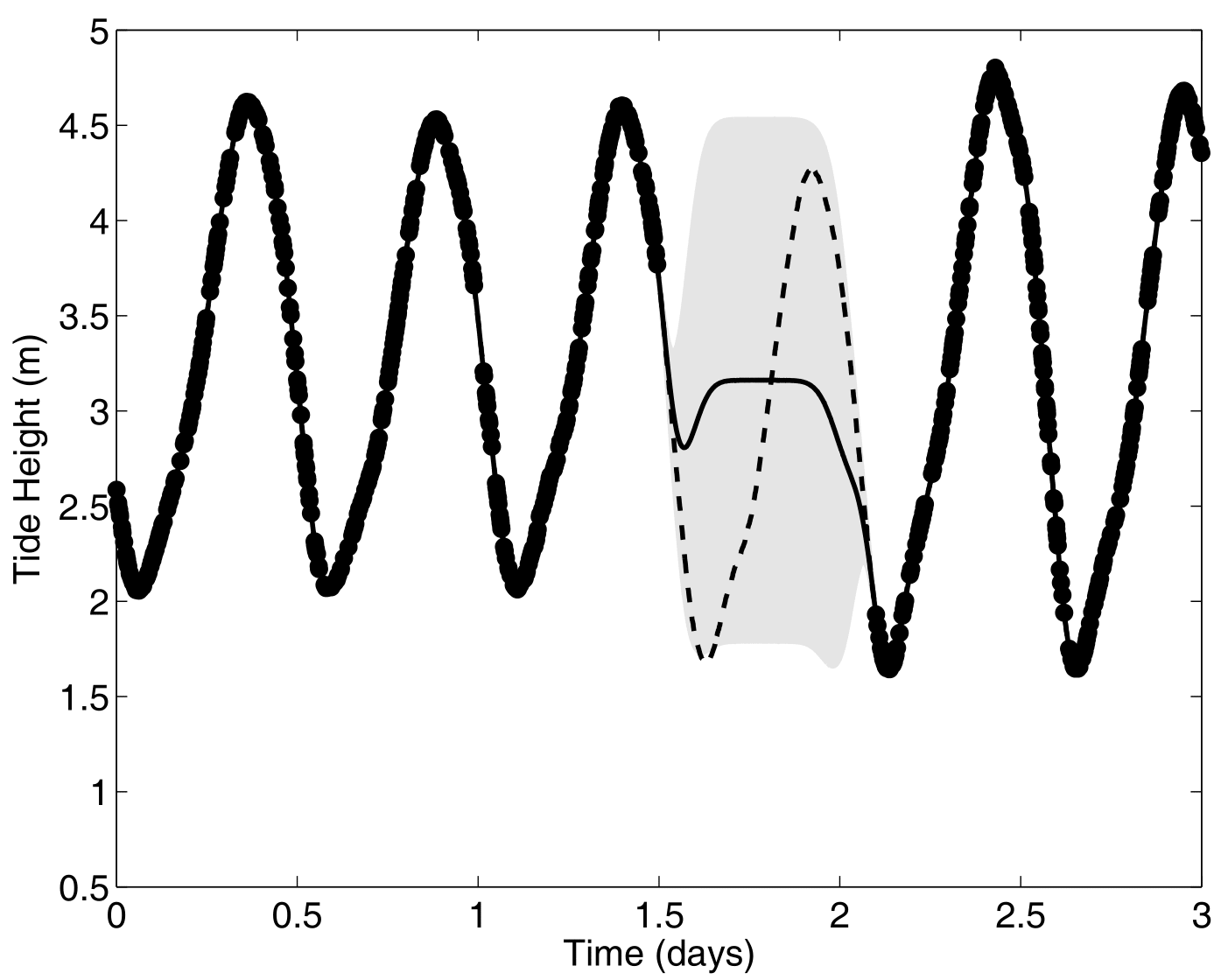
Forecasting with a unique GP

Forecasting with a unique GP

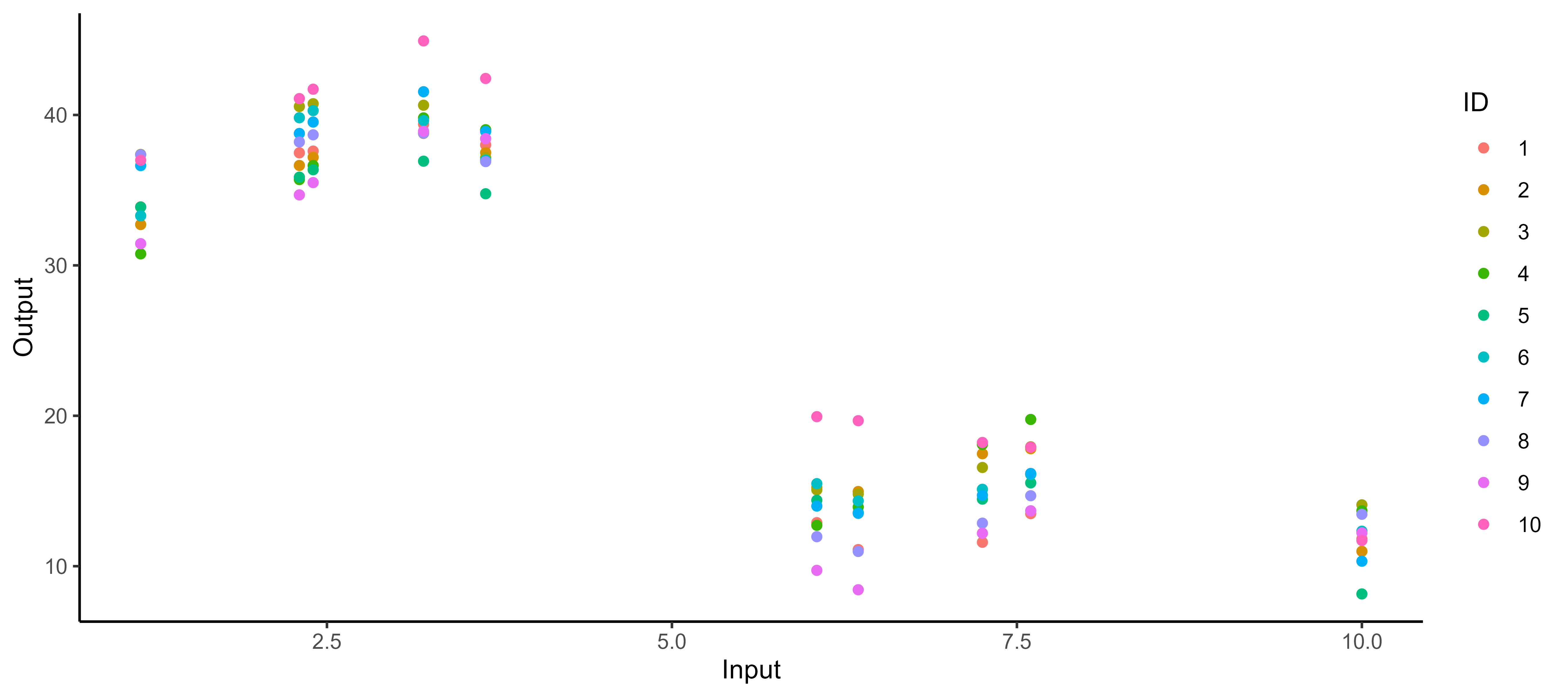
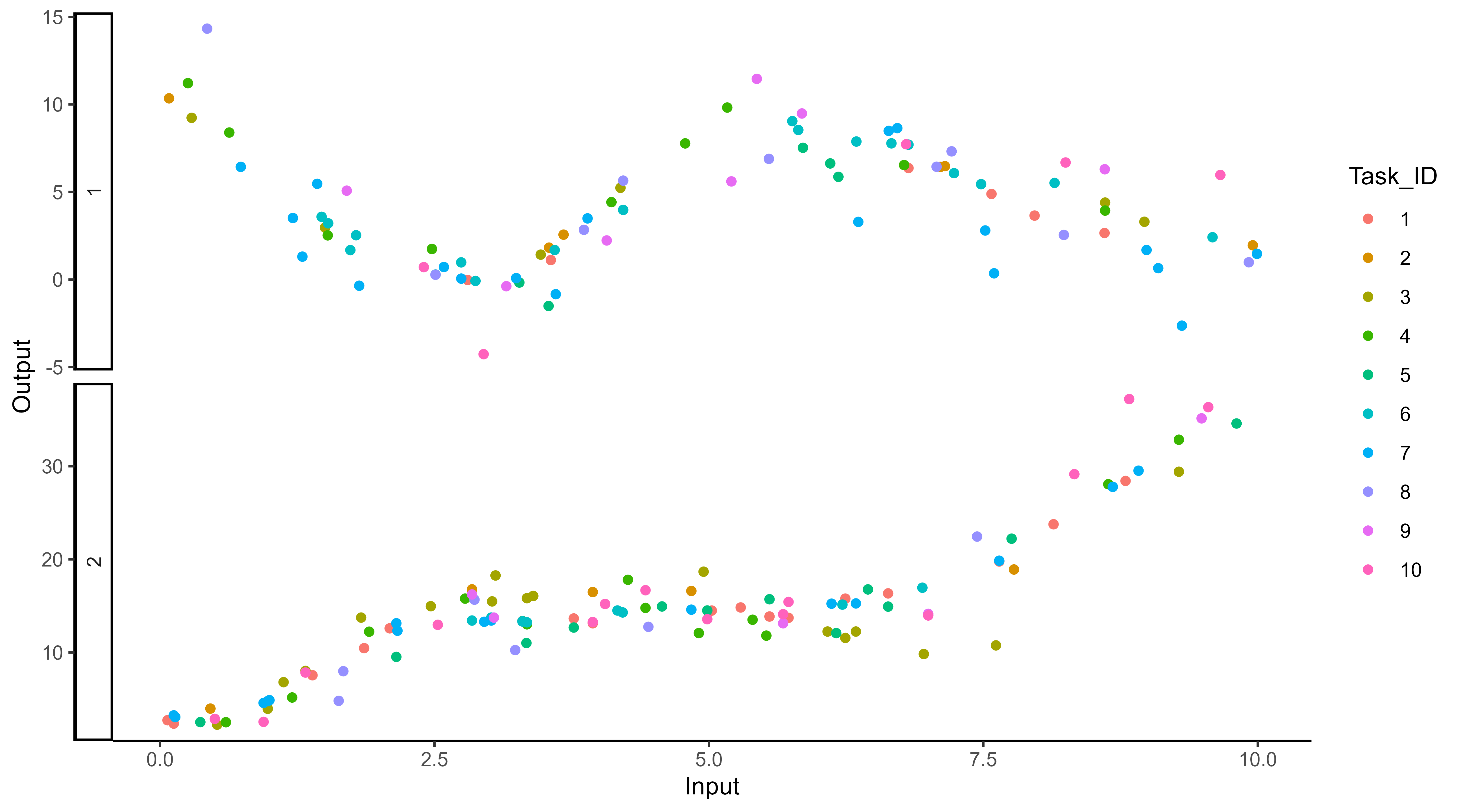
It all starts with observations from multiple sources …

The real journey starts with observations from multiple sources …

… but sometimes we are not measuring the same things …

… and the input space can be multidimensional as well …

… among many other difficulties …

Several classical challenges:

• Irregular measurements (in number of observations and location),

… among many other difficulties …

Several classical challenges:

• Irregular measurements (in number of observations and location),
  
• Multiple sources of data (individuals, sensors, …)

… or all of them at once!

Multi-Task? Multi-Output? What are the maths behind that?

In the previous examples, we saw a variety of situations that naturally lead to the same mathematical formulation of the learning problem:

\[y_s = \color{orange}{f_s}(x_s) + \epsilon_s, \hspace{3cm} \forall s = 1, \dots, S\]

Learn \(\color{orange}{f_s}\), the underlying relationship between \(x_s\) and \(y_s\), for each source of data \(\color{orange}{s}\).

Multi-, in contrast with single-, regression implies that some information can be shared across data sources to improve learning/predictions.

The nature of measurements leads to a more philosophical distinction:

• Multi-Output clearly refers to several variables of interest. An Output is a quantity we aim to infer/predict from Input measurements, and which may be correlated with others.
• Multi-Task implies the existence of an underlying pattern, shared by several tasks or individuals, which can be jointly exploited to build a common model.

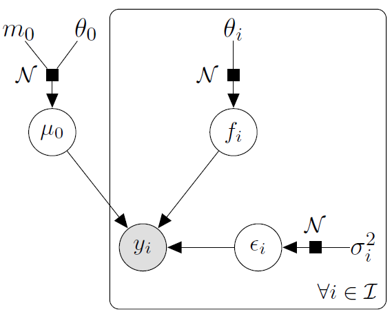
Multi-Task Gaussian Processes

\[y_t = \mu_0 + f_t + \epsilon_t, \hspace{3cm} \forall t = 1, \dots, T\]

with:

• \(\mu_0 \sim \mathcal{GP}(m_0, K_{0}),\)
• \(f_t \sim \mathcal{GP}(0, \Sigma_{\theta_t}), \ \perp \!\!\! \perp_t,\)
• \(\epsilon_t \sim \mathcal{GP}(0, \sigma_t^2), \ \perp \!\!\! \perp_t.\)

It follows that:

\[y_t \mid \mu_0 \sim \mathcal{GP}(\mu_0, \Sigma_{\theta_t} + \sigma_t^2 I), \ \perp \!\!\! \perp_t\]

\(\rightarrow\) Unified GP framework with a shared mean process \(\mu_0\), and task-specific process \(f_t\),
\(\rightarrow\) Naturaly handles irregular grids of input data.

Goal: Learn the hyper-parameters, (and \(\mu_0\)’s hyper-posterior).
Difficulty: The likelihood depends on \(\mu_0\), and tasks are not independent.

EM algorithm

E-step

\[ \begin{align} p(\mu_0(\color{grey}{\mathbf{x}}) \mid \textbf{y}, \hat{\Theta}) &\propto \mathcal{N}(\mu_0(\color{grey}{\mathbf{x}}); m_0(\color{grey}{\textbf{x}}), \textbf{K}_{0}^{\color{grey}{\textbf{x}}}) \times \prod\limits_{t =1}^T \mathcal{N}(\mathbf{y}_t; \mu_0( \color{purple}{\textbf{x}_i}), \boldsymbol{\Psi}_{\hat{\theta}_i, \hat{\sigma}_i^2}^{\color{purple}{\textbf{x}_i}}) \\ &= \mathcal{N}(\mu_0(\color{grey}{\mathbf{x}}); \hat{m}_0(\color{grey}{\textbf{x}}), \hat{\textbf{K}}^{\color{grey}{\textbf{x}}}), \end{align} \]

• \(\hat{\textbf{K}}^{\color{grey}{\textbf{x}}} = ({\textbf{K}_{0}^{\color{grey}{\textbf{x}}}}^{-1} + \sum\limits_{t = 1}^T {\boldsymbol{\Psi}_{\hat{\theta}_i, \hat{\sigma}_i^2}^{\color{purple}{\textbf{x}_i}}}^{-1})^{-1}\)
• \(\hat{m}_0(\color{grey}{\textbf{x}}) = \hat{\textbf{K}}^{\color{grey}{\textbf{x}}}({\textbf{K}_{0}^{\color{grey}{\textbf{x}}}}^{-1} m_0(\color{grey}{\mathbf{x}}) + \sum\limits_{t = 1}^T {\boldsymbol{\Psi}_{\hat{\theta}_i, \hat{\sigma}_i^2}^{\color{purple}{\textbf{x}_i}}}^{-1} \mathbf{y}_t)\).

M-step

\[ \begin{align*} \hat{\Theta} &= \underset{\Theta}{\arg\max} \ \ \sum\limits_{t = 1}^{T}\left\{ \log \mathcal{N} \left( \mathbf{y}_t; \hat{m}_0(\color{purple}{\mathbf{x}_t}), \boldsymbol{\Psi}_{\theta_t, \sigma^2}^{\color{purple}{\mathbf{x}_t}} \right) - \dfrac{1}{2} Tr \left( \hat{\mathbf{K}}^{\color{purple}{\mathbf{x}_t}} {\boldsymbol{\Psi}_{\theta_t, \sigma^2}^{\color{purple}{\mathbf{x}_t}}}^{-1} \right) \right\}. \end{align*} \]

Covariance structure assumption and computational complexity

Sharing the covariance structures or not offers a compromise between flexibility and parsimony:

• One optimisation problem for \(\theta\), and a shared process for all tasks,
  
• \(\color{blue}{T}\) distinct optimisation problems for \(\{\theta_t\}_t\), and task-specific processes.

Major interests:

• Both approaches scale linearly with the number of tasks,
  
• Parallel computing can be used to speed up training.

Overall, the computational complexity is: \[ \mathcal{O}(\color{blue}{T} \times N_t^3 + N^3) \]

with \(N = \bigcup\limits_{t = 1}^\color{blue}{T} N_t\)

Predictions with Multi-Task GPs

• Multi-Task prior:

\[p \left( \begin{bmatrix} y_*(\color{grey}{\mathbf{x}_{*}}) \\ y_*(\color{purple}{\mathbf{x}^{p}}) \\ \end{bmatrix} \mid \textbf{y} \right) = \mathcal{N} \left( \begin{bmatrix} y_*(\color{grey}{\mathbf{x}_{*}}) \\ y_*(\color{purple}{\mathbf{x}^{p}}) \\ \end{bmatrix}; \ \begin{bmatrix} \hat{m}_0(\color{grey}{\mathbf{x}_{*}}) \\ \hat{m}_0(\color{purple}{\mathbf{x}^{p}}) \\ \end{bmatrix}, \begin{pmatrix} \Gamma_{\color{grey}{**}} & \Gamma_{\color{grey}{*}\color{purple}{p}} \\ \Gamma_{\color{purple}{p}\color{grey}{*}} & \Gamma_{\color{purple}{pp}} \end{pmatrix} \right)\]

• Multi-Task posterior:

\[p(y_*(\color{purple}{\mathbf{x}^{p}}) \mid y_*(\color{grey}{\mathbf{x}_{*}}), \textbf{y}) = \mathcal{N} \Big( y_*(\color{purple}{\mathbf{x}^{p}}); \ \hat{\mu}_{*}(\color{purple}{\mathbf{x}^{p}}) , \hat{\Gamma}_{\color{purple}{pp}} \Big)\]

with:

• \(\hat{\mu}_{*}(\color{purple}{\mathbf{x}^{p}}) = \hat{m}_0(\color{purple}{\mathbf{x}^{p}}) + \Gamma_{\color{purple}{p}\color{grey}{*}}\Gamma_{\color{grey}{**}}^{-1} (y_*(\color{grey}{\mathbf{x}_{*}}) - \hat{m}_0 (\color{grey}{\mathbf{x}_{*}}))\)
• \(\hat{\Gamma}_{\color{purple}{pp}} = \Gamma_{\color{purple}{pp}} - \Gamma_{\color{purple}{p}\color{grey}{*}}\Gamma_{\color{grey}{**}}^{-1} \Gamma_{\color{grey}{*}\color{purple}{p}}\)

A GIF is worth a thousand words

A GIF is worth a thousand words

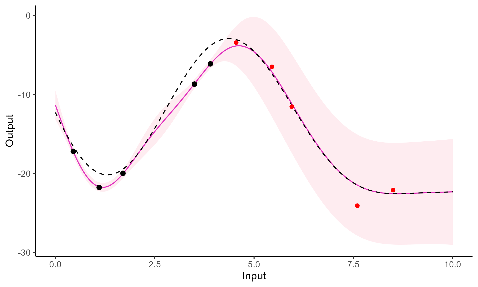
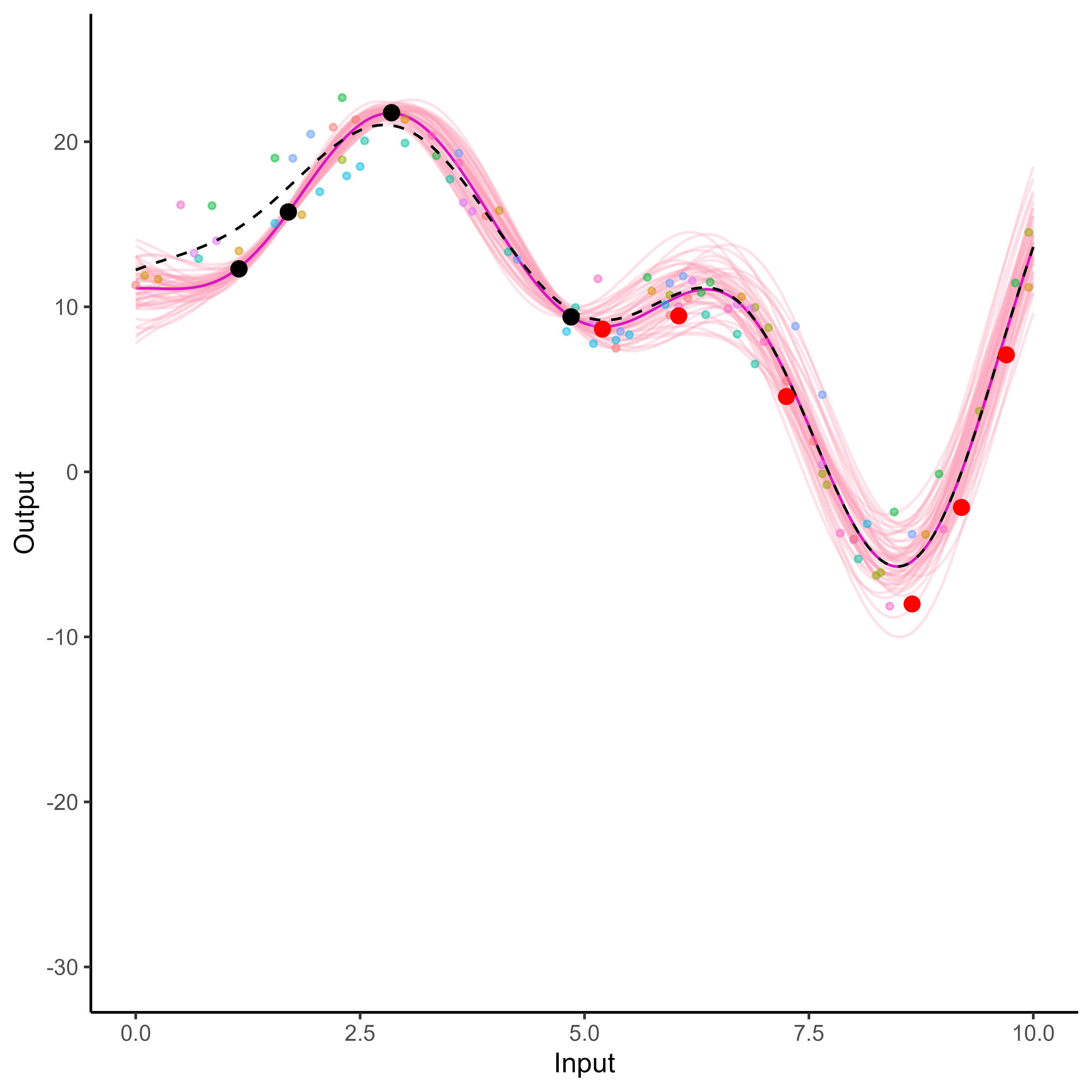
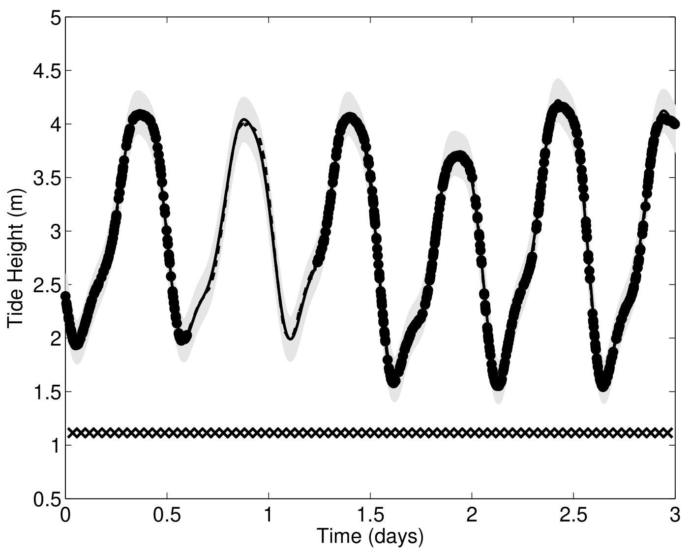
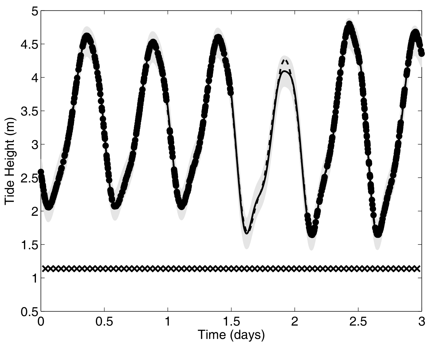
Comparison with single GP regression

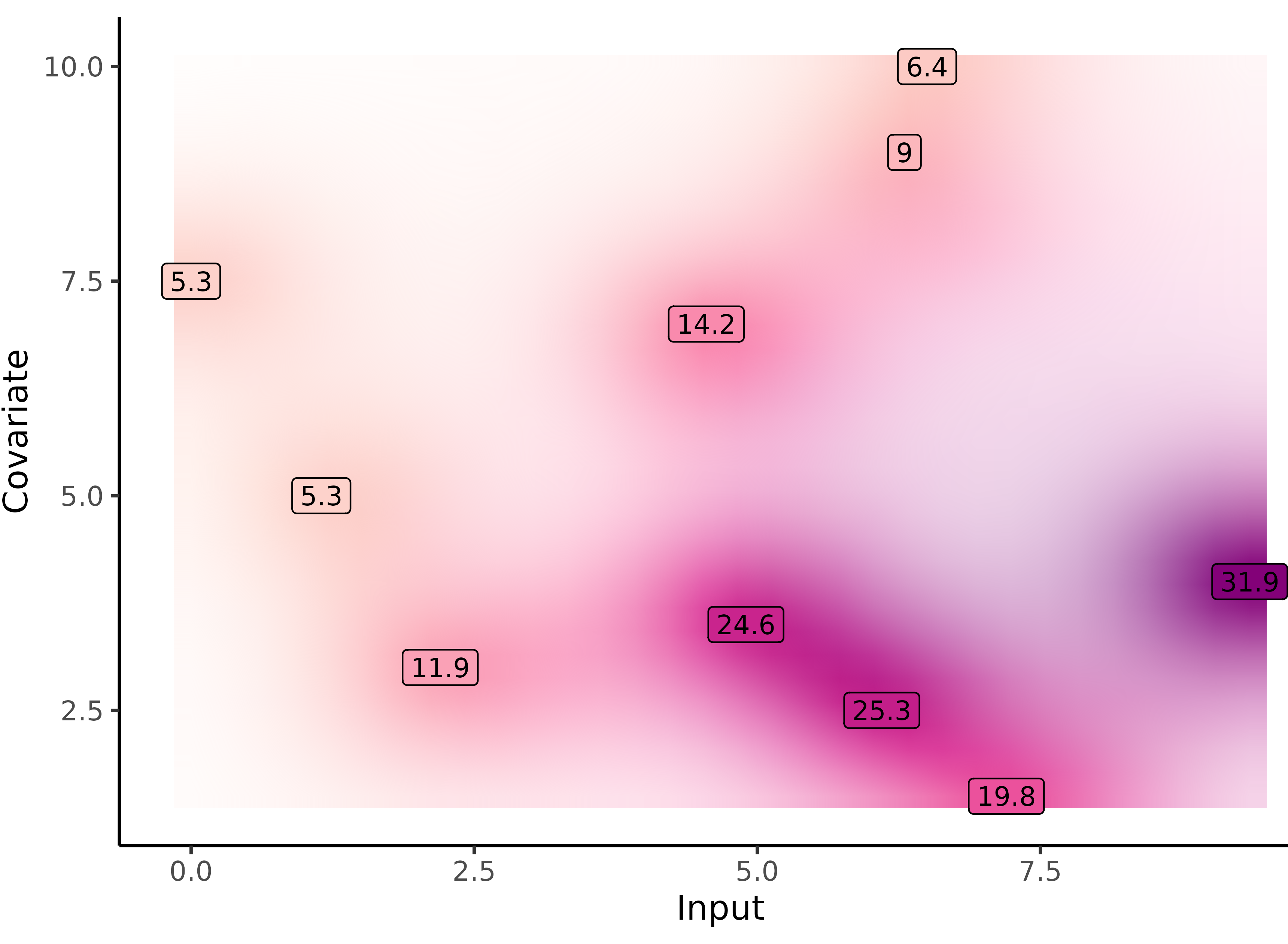
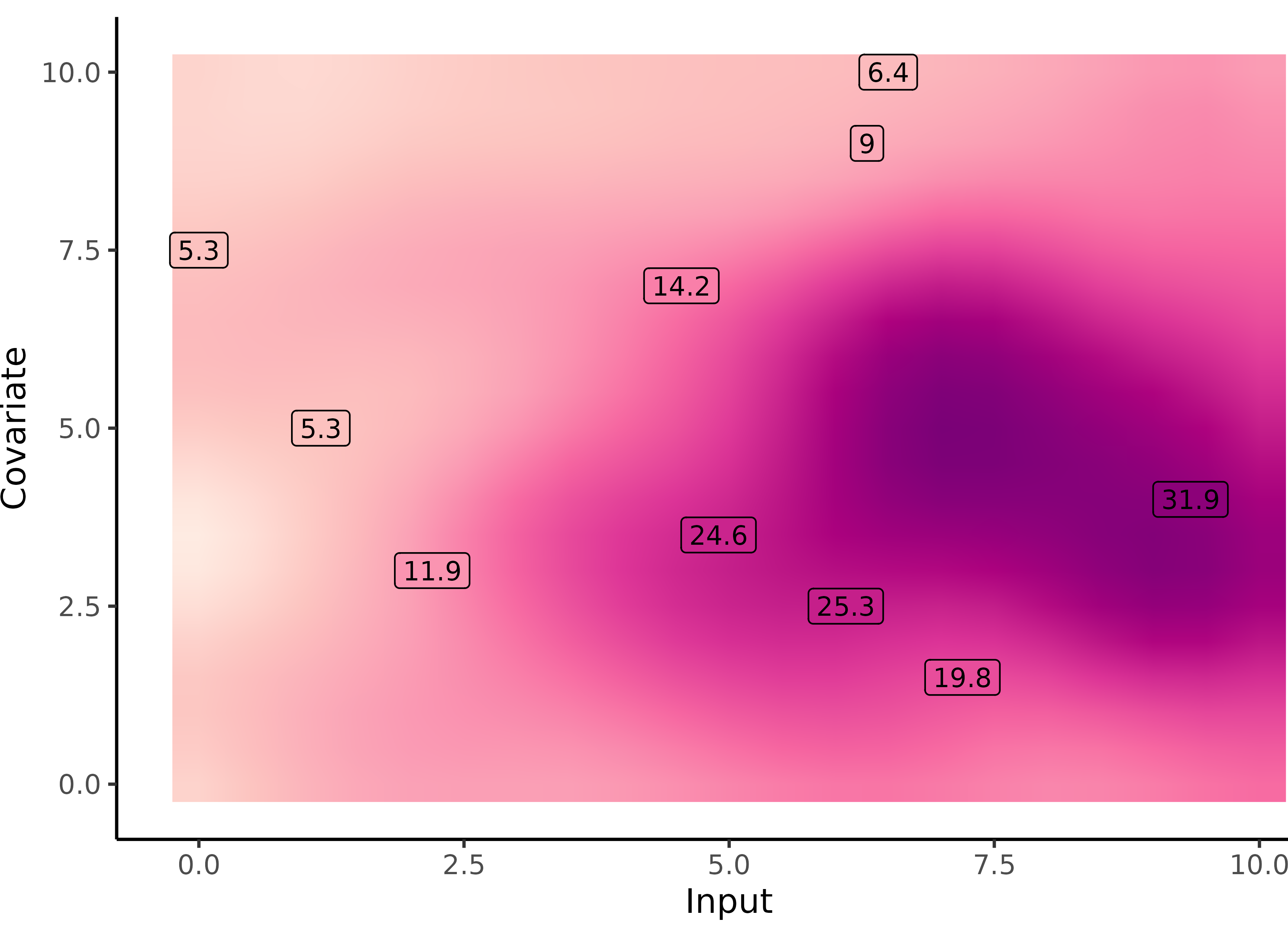
Yet another comparison with single GP regression but in 2D

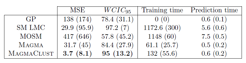
Multi-Task GPs regression provides more reliable predictions when individual processes are sparsely observed, while greatly reducing the associated uncertainty

Adding some clustering into Multi-Task GPs

A unique underlying mean process might be too restrictive.

\(\rightarrow\) Mixture of multi-task GPs:

\[y_t = \mu_0 + f_t + \epsilon_t, \hspace{3cm} \forall t = 1, \dots, T\]

with:

• \(\color{green}{Z_{t}} \sim \mathcal{M}(1, \color{green}{\boldsymbol{\pi}}), \ \perp \!\!\! \perp_t,\)

• \(\mu_0 \sim \mathcal{GP}(m_0, K_0),\)
• \(f_t \sim \mathcal{GP}(0, \Sigma_{\theta_t}), \ \perp \!\!\! \perp_t,\)
• \(\epsilon_t \sim \mathcal{GP}(0, \sigma_t^2), \ \perp \!\!\! \perp_t.\)

It follows that:

\[y_t \mid \mu_0 \sim \mathcal{GP}(\mu_0, \Psi_t), \ \perp \!\!\! \perp_t\]

Adding some clustering into Multi-Task GPs

A unique underlying mean process might be too restrictive.

\(\rightarrow\) Mixture of multi-task GPs:

\[y_t \mid \{\color{green}{Z_{tk}} = 1 \} = \mu_{\color{green}{k}} + f_t + \epsilon_t, \hspace{3cm} \forall t = 1, \dots, T\]

with:

• \(\color{green}{Z_{t}} \sim \mathcal{M}(1, \color{green}{\boldsymbol{\pi}}), \ \perp \!\!\! \perp_t,\)
• \(\mu_{\color{green}{k}} \sim \mathcal{GP}(m_{\color{green}{k}}, \color{green}{C_{{k}}})\ \perp \!\!\! \perp_{\color{green}{k}},\)
• \(f_t \sim \mathcal{GP}(0, \Sigma_{\theta_t}), \ \perp \!\!\! \perp_t,\)
• \(\epsilon_t \sim \mathcal{GP}(0, \sigma_t^2), \ \perp \!\!\! \perp_t.\)

It follows that:

\[y_t \mid \mu_0 \sim \mathcal{GP}(\mu_0, \Psi_t), \ \perp \!\!\! \perp_t\]

Adding some clustering into Multi-Task GPs

A unique underlying mean process might be too restrictive.

\(\rightarrow\) Mixture of multi-task GPs:

\[y_t \mid \{\color{green}{Z_{ik}} = 1 \} = \mu_{\color{green}{k}} + f_t + \epsilon_t, \hspace{3cm} \forall t = 1, \dots, T\]

with:

• \(\color{green}{Z_{t}} \sim \mathcal{M}(1, \color{green}{\boldsymbol{\pi}}), \ \perp \!\!\! \perp_t,\)
• \(\mu_{\color{green}{k}} \sim \mathcal{GP}(m_{\color{green}{k}}, \color{green}{C_{{k}}})\ \perp \!\!\! \perp_{\color{green}{k}},\)
• \(f_t \sim \mathcal{GP}(0, \Sigma_{\theta_t}), \ \perp \!\!\! \perp_t,\)
• \(\epsilon_t \sim \mathcal{GP}(0, \sigma_t^2), \ \perp \!\!\! \perp_t.\)

It follows that:

\[y_t \mid \{ \boldsymbol{\mu} , \color{green}{\boldsymbol{\pi}} \} \sim \sum\limits_{k=1}^K{ \color{green}{\pi_k} \ \mathcal{GP}\Big(\mu_{\color{green}{k}}, \Psi_t^\color{green}{k} \Big)}, \ \perp \!\!\! \perp_t\]

Variational EM

E step: \[ \begin{align} \hat{q}_{\boldsymbol{\mu}}(\boldsymbol{\mu}) &= \color{green}{\prod\limits_{k = 1}^K} \mathcal{N}(\mu_\color{green}{k};\hat{m}_\color{green}{k}, \hat{\textbf{C}}_\color{green}{k}) , \hspace{2cm} \hat{q}_{\boldsymbol{Z}}(\boldsymbol{Z}) = \prod\limits_{t = 1}^T \mathcal{M}(Z_t;1, \color{green}{\boldsymbol{\tau}_t}) \end{align} \] M step:

\[ \begin{align*} \hat{\Theta} &= \underset{\Theta}{\arg\max} \sum\limits_{k = 1}^{K}\sum\limits_{t = 1}^{T}\tau_{tk}\ \mathcal{N} \left( \mathbf{y}_t; \ \hat{m}_k, \boldsymbol{\Psi}_{\color{blue}{\theta_t}, \color{blue}{\sigma_t^2}} \right) - \dfrac{1}{2} \textrm{tr}\left( \mathbf{\hat{C}}_k\boldsymbol{\Psi}_{\color{blue}{\theta_t}, \color{blue}{\sigma_t^2}}^{-1}\right) \\ & \hspace{1cm} + \sum\limits_{k = 1}^{K}\sum\limits_{t = 1}^{T}\tau_{tk}\log \color{green}{\pi_{k}} \end{align*} \]

Cluster-specific and mixture predictions

• Multi-Task posterior for each cluster:

\[ p(y_*(\mathbf{x}^{p}) \mid \color{green}{Z_{*k}} = 1, y_*(\mathbf{x}_{*}), \textbf{y}) = \mathcal{N} \Big( y_*(\mathbf{x}^{p}); \ \hat{\mu}_{*}^\color{green}{k}(\mathbf{x}^{p}) , \hat{\Gamma}_{pp}^\color{green}{k} \Big), \forall \color{green}{k}, \]

\(\hat{\mu}_{*}^\color{green}{k}(\mathbf{x}^{p}) = \hat{m}_\color{green}{k}(\mathbf{x}^{p}) + \Gamma^\color{green}{k}_{p*} {\Gamma^\color{green}{k}_{**}}^{-1} (y_*(\mathbf{x}_{*}) - \hat{m}_\color{green}{k} (\mathbf{x}_{*}))\)
\(\hat{\Gamma}_{pp}^\color{green}{k} = \Gamma_{pp}^\color{green}{k} - \Gamma_{p*}^\color{green}{k} {\Gamma^{\color{green}{k}}_{**}}^{-1} \Gamma^{\color{green}{k}}_{*p}\)

• Predictive multi-task GPs mixture:

\[p(y_*(\textbf{x}^p) \mid y_*(\textbf{x}_*), \textbf{y}) = \color{green}{\sum\limits_{k = 1}^{K} \tau_{*k}} \ \mathcal{N} \big( y_*(\mathbf{x}^{p}); \ \hat{\mu}_{*}^\color{green}{k}(\textbf{x}^p) , \hat{\Gamma}_{pp}^\color{green}{k}(\textbf{x}^p) \big).\]

An image is still worth many words

A unique mean process can struggle to capture relevant signals in presence of group structures.

An image is still worth many words

By identifying the underlying clustering structure, we can discard unnecessary information and provide enhanced predictions as well as lower uncertainty.

Saved by the weights

Each cluster-specific prediction is weighted by its membership probability \(\color{green}{\tau_{*k}}\).

Performance of MagmaClust

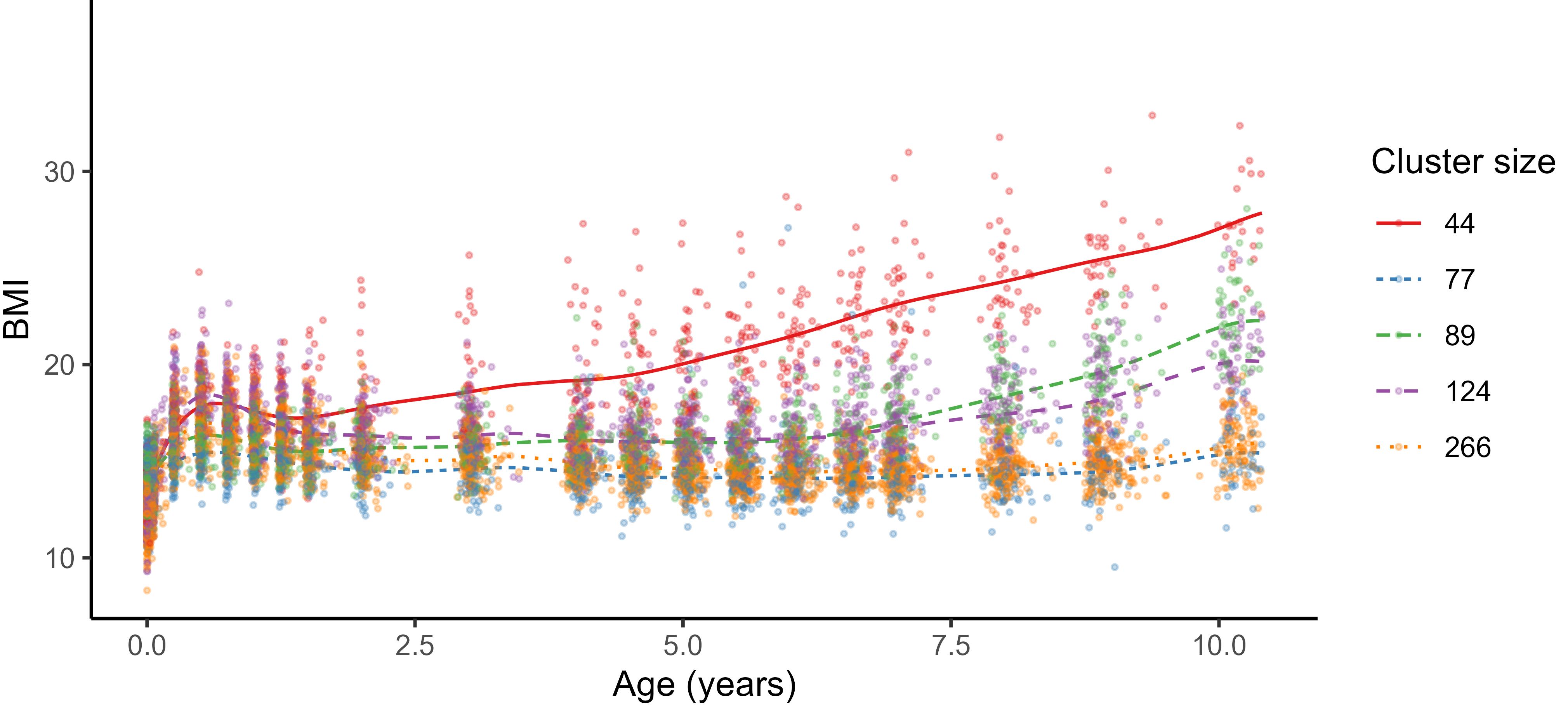
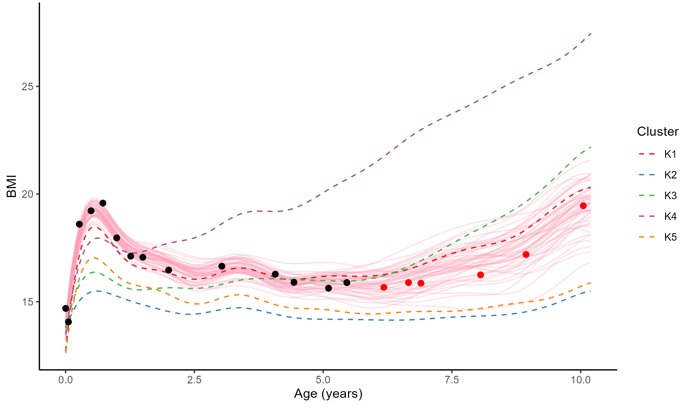
Practical application: follow up of BMI during childhood

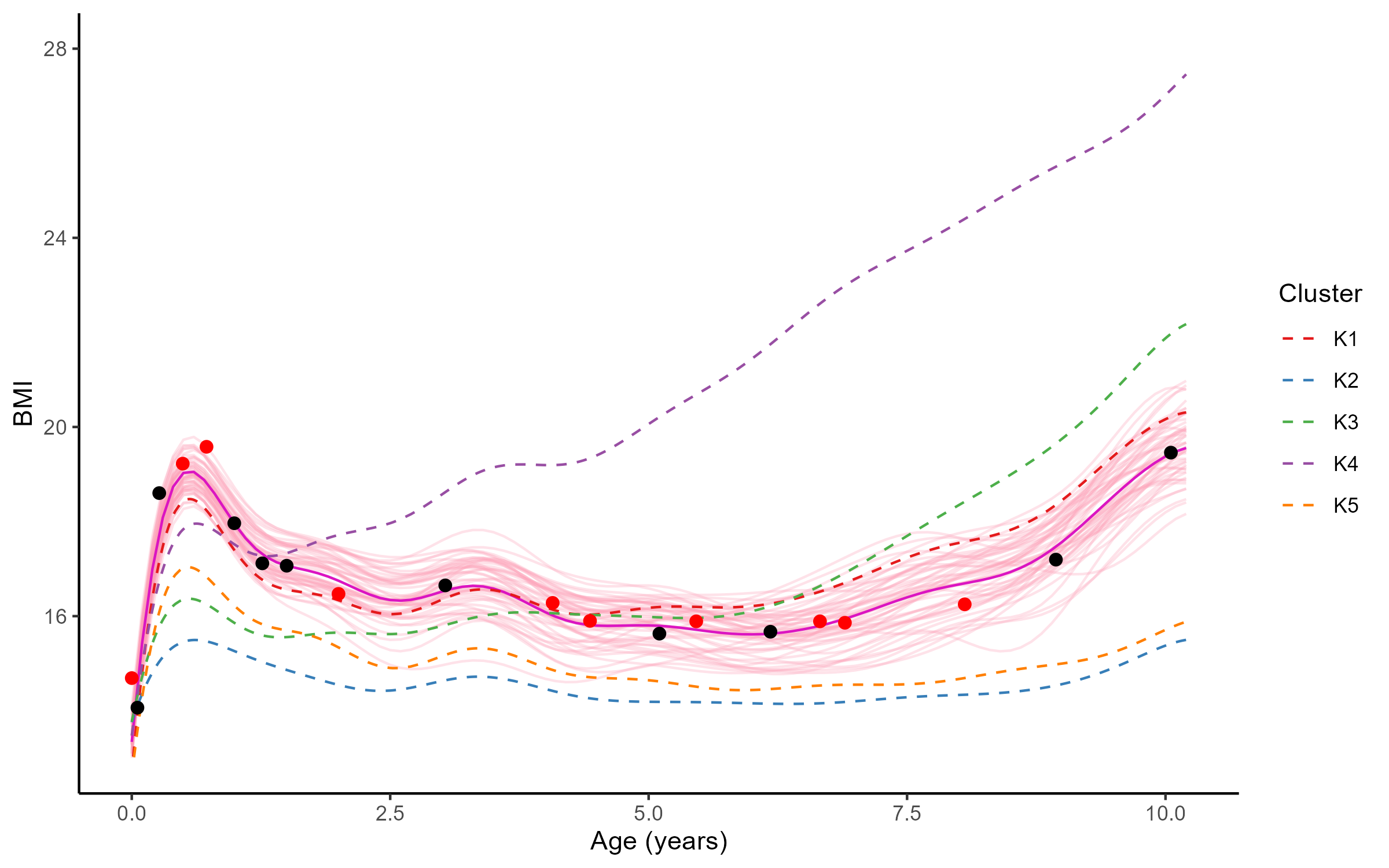
Reconstruction for sparse or incomplete data

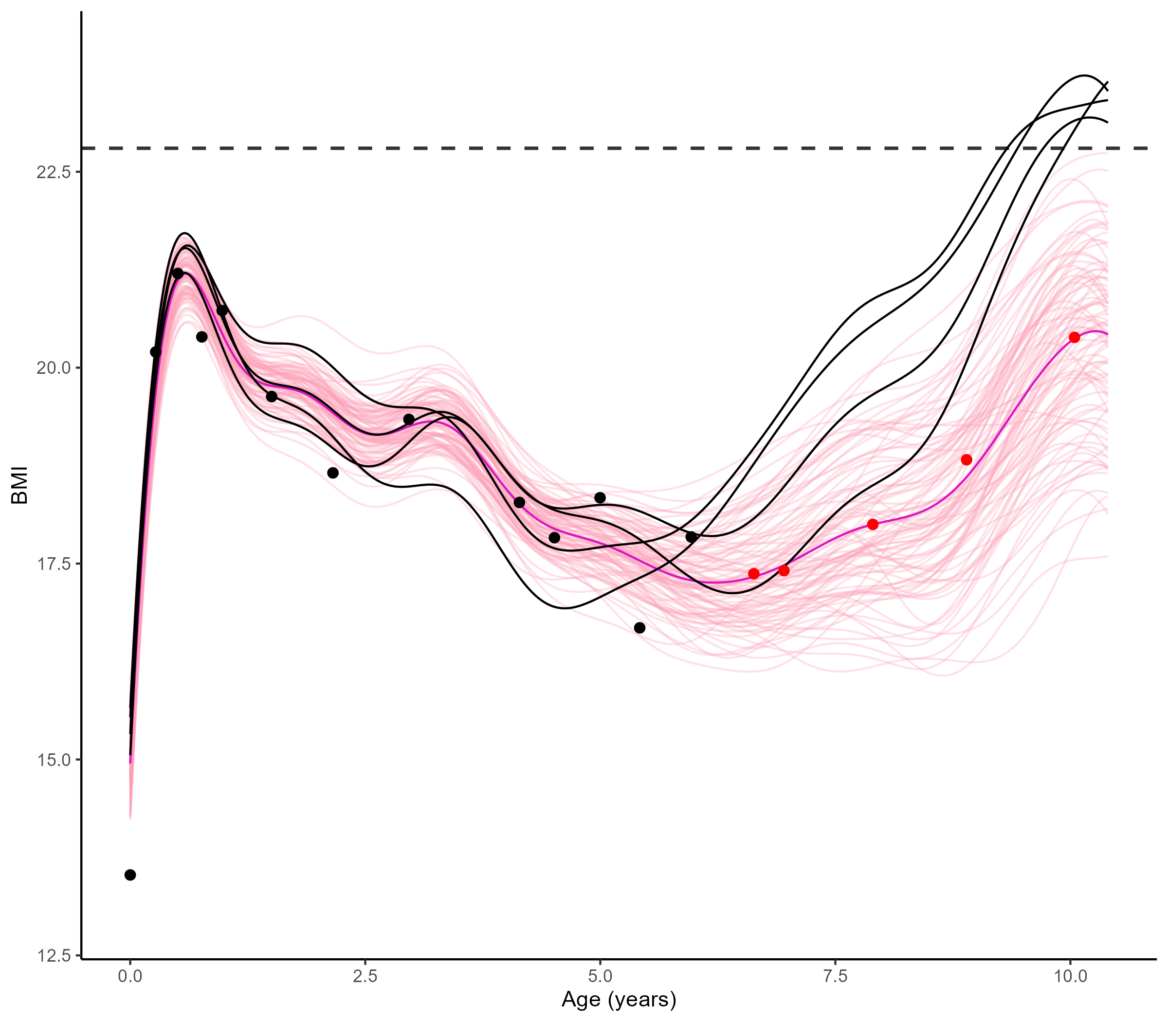
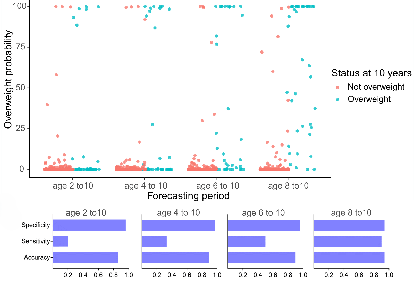
Forecasting long term evolution of BMI

Leveraging the uncertainty quantification of GPs

Deriving downstream tools for practitioners

Uncertainty quantification provides valuable information to practitioners to make decisions based on probabilistic statements, like the risk of overweight at 10 years.

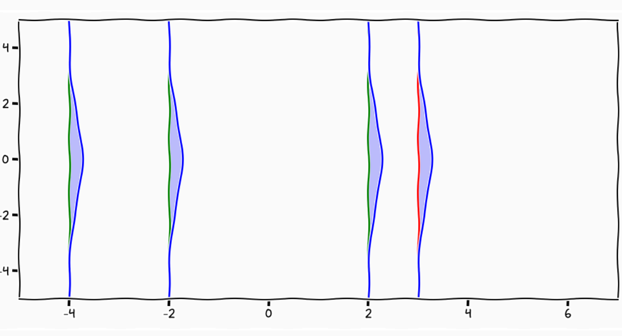
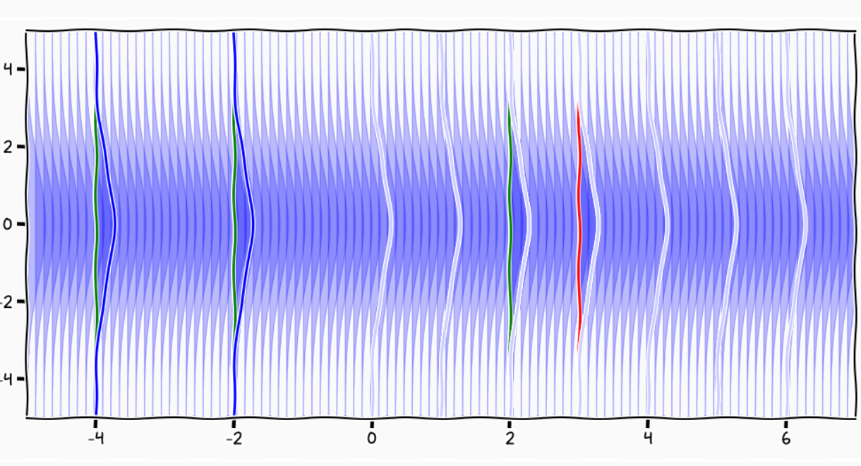
Multi-Output GPs: another paradigm based on covariance structures

Multi-Task-Multi-Output GPs: best of both worlds?

• Multi-Output GPs derive full rank covariance matrices to exploit cross-correlations between all Input-Output pairs. They are flexible, expressive, and well-designed to recover very different signals or measurements. On the down side, they are computationally expensive, sometimes difficult to train in practice, and poorly adapted to modelling multiple tasks/individuals.

• Multi-Task GPs leverage latent mean processes to share information on the common trends and properties of the data. They are parsimonious, efficient, and well-designed to capture common patterns for multiple tasks/individuals on the same variable of interest. On the down side, they can be limited to fully capture correlations between the GPs and exploit initial knowledge that collected data may be of different natures.

Both work on separate parts of a GP, with no assumption on the other, and are theoretically compatible. They are even expected to synergise well, by tackling each others limitations.

Generative model of MOMT GPs

\[\begin{bmatrix} y_t^{1} \\ \vdots \\ y_t^{O} \\ \end{bmatrix} = \begin{bmatrix} \mu_0 \\ \vdots \\ \mu_0 \\ \end{bmatrix} + \begin{bmatrix} f_t^{1} \\ \vdots \\ f_t^{O} \\ \end{bmatrix} + \begin{bmatrix} \epsilon_t^{1} \\ \vdots \\ \epsilon_t^{O} \\ \end{bmatrix}, \hspace{3cm} \forall t = 1, \dots, T\]

• \(\mu_0 \sim \mathcal{GP}(m_0, K_0),\)
• \(\begin{bmatrix} f_t^{1} \\ \vdots \\ f_t^{O} \\ \end{bmatrix} \sim \mathcal{GP}(0, \Sigma_{\theta_t}), \ \perp \!\!\! \perp_t,\)
• \(\begin{bmatrix} \epsilon_t^{1} \\ \vdots \\ \epsilon_t^{O} \\ \end{bmatrix} \sim \mathcal{GP}(0, \begin{bmatrix} {\sigma_t^{1}}^O \\ \vdots \\ {\sigma_{t}^O}^2 \\ \end{bmatrix} \times I_O), \ \perp \!\!\! \perp_t.\)

All mathematical objects from Multi-Task GPs are now extended with stacked Outputs.

Process convolution covariance structure and inference

\[\Big[k_{\theta_t}(\mathbf{x}, \mathbf{x}^{\prime})\Big]_{o,o'} = \dfrac{S_{t,o} \ S_{t,o{\prime}}}{(2\pi)^{D/2} \ |\Sigma|^{1/2}} \ \exp\Big(-\dfrac{1}{2}(\mathbf{x} - \mathbf{x}^{\prime})^T \Sigma^{-1}(\mathbf{x}-\mathbf{x}^{\prime})\Big)\]

with:

• \(S_{t,o}, S_{t,o{\prime}} \in \mathbb{R}\), the Output-specific variance terms,
• \(\Sigma = P_{t,o}^{-1}+P_{t,o^{\prime}}^{-1}+\Lambda^{-1} \in \mathbb{R}^{D \times D}\).

These matrices are typically diagonal, filled with Output-specific and latent lengthscales, one per Input dimension. In the end, we need to optimise \(\color{red}{O}\times \color{blue}{T} \times (3D+1)\) hyper-parameters.

E-step

\[ \begin{align} p(\mu_0(\color{grey}{\mathbf{x}}) \mid \textbf{y}, \hat{\Theta}) = \mathcal{N}(\mu_0(\color{grey}{\mathbf{x}}); \hat{m}_0(\color{grey}{\textbf{x}}), \hat{\textbf{K}}^{\color{grey}{\textbf{x}}}), \end{align} \]

M-step

\[ \begin{align*} \hat{\Theta} &= \underset{\Theta}{\arg\max} \sum\limits_{t = 1}^{T}\left\{ \log \mathcal{N} \left( \mathbf{y}_t; \hat{m}_0(\color{purple}{\mathbf{x}_t^O}), \boldsymbol{\Psi}_{\theta_t, \sigma_t^2}^{\color{purple}{\mathbf{x}_t^O}} \right) - \dfrac{1}{2} Tr \left( \hat{\mathbf{K}}^{\color{purple}{\mathbf{x}_t^O}} {\boldsymbol{\Psi}_{\theta_t, \sigma_t^2}^{\color{purple}{\mathbf{x}_t^O}}}^{-1} \right) \right\}. \end{align*} \]

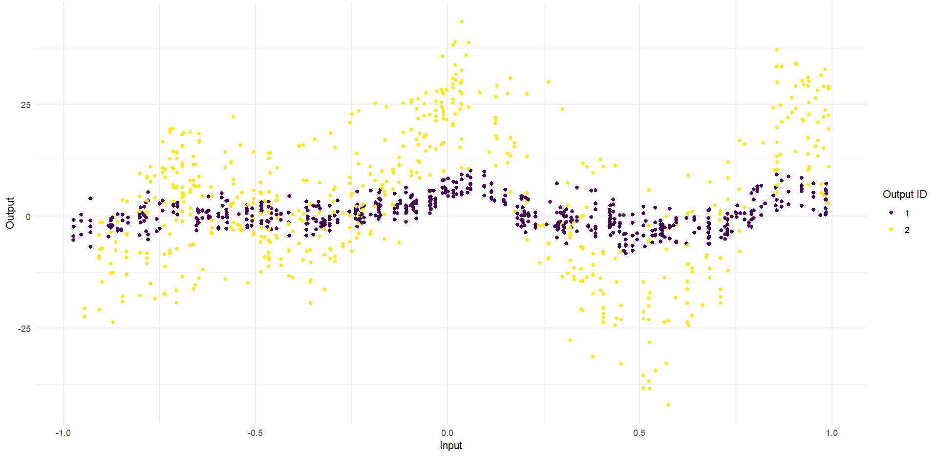
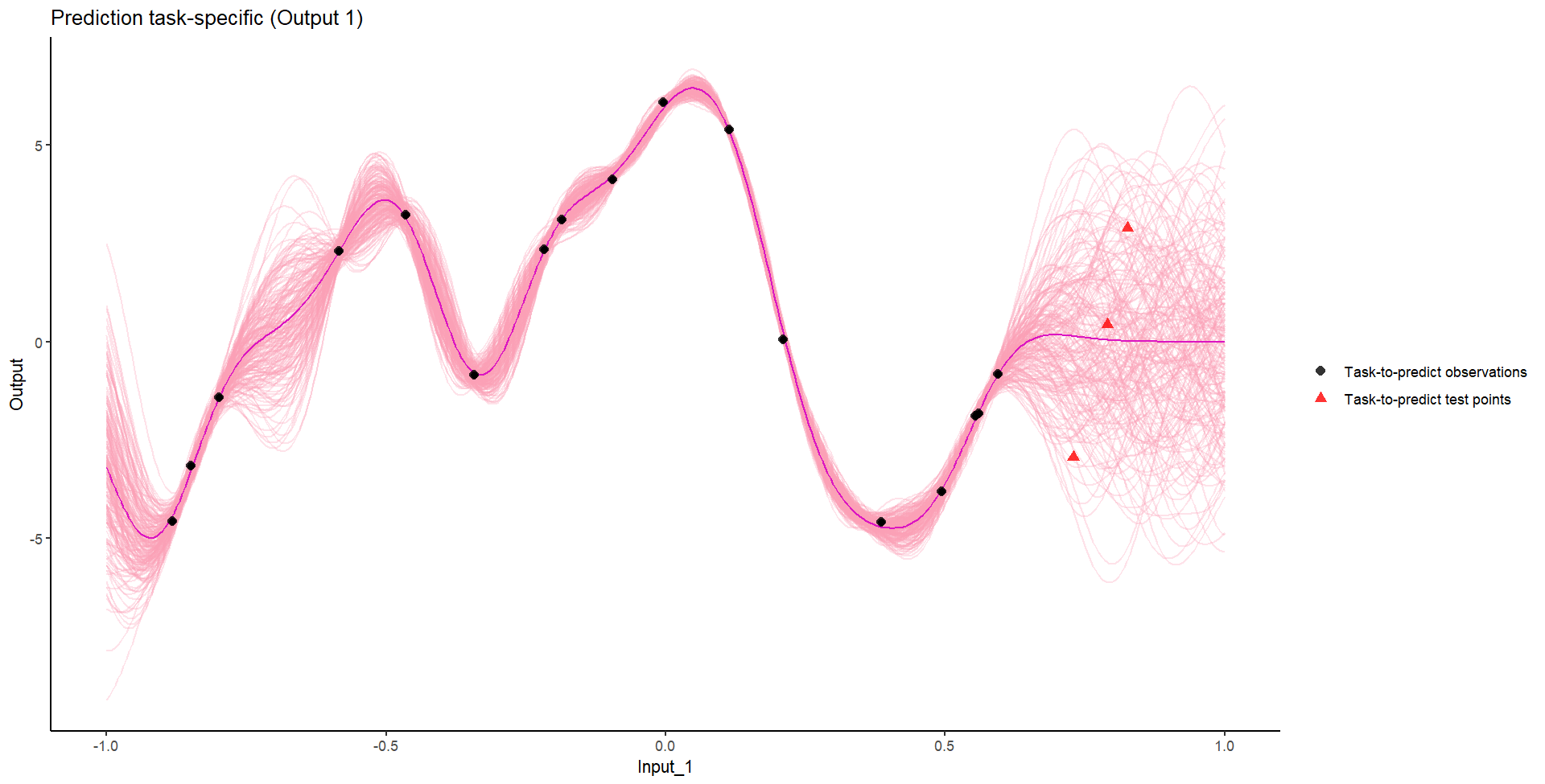
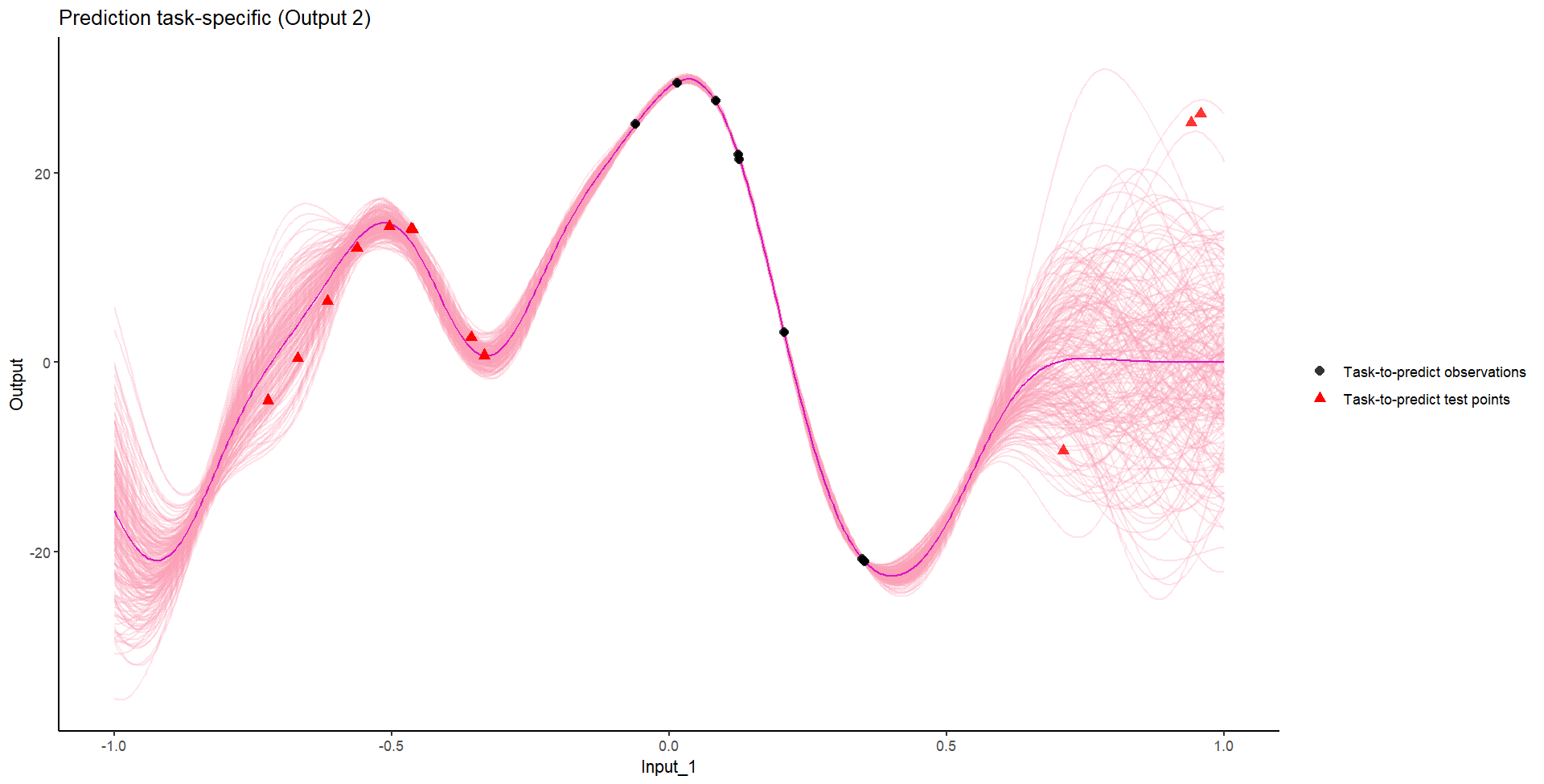
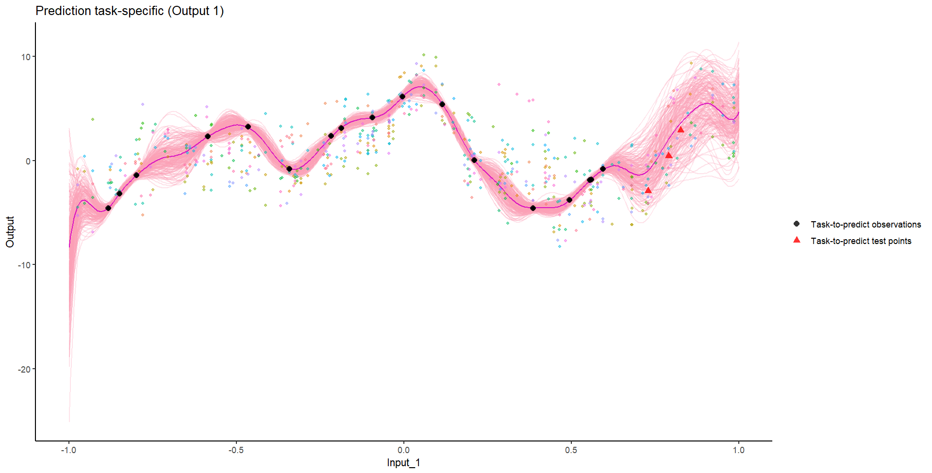
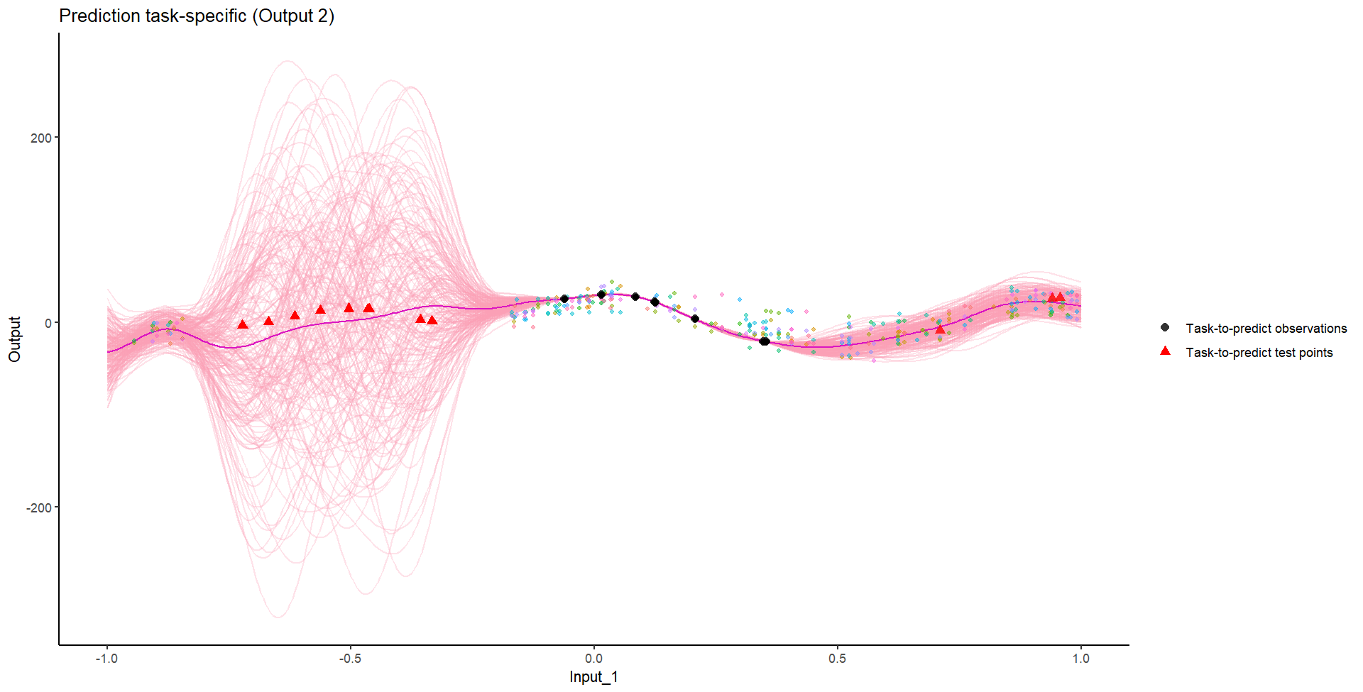
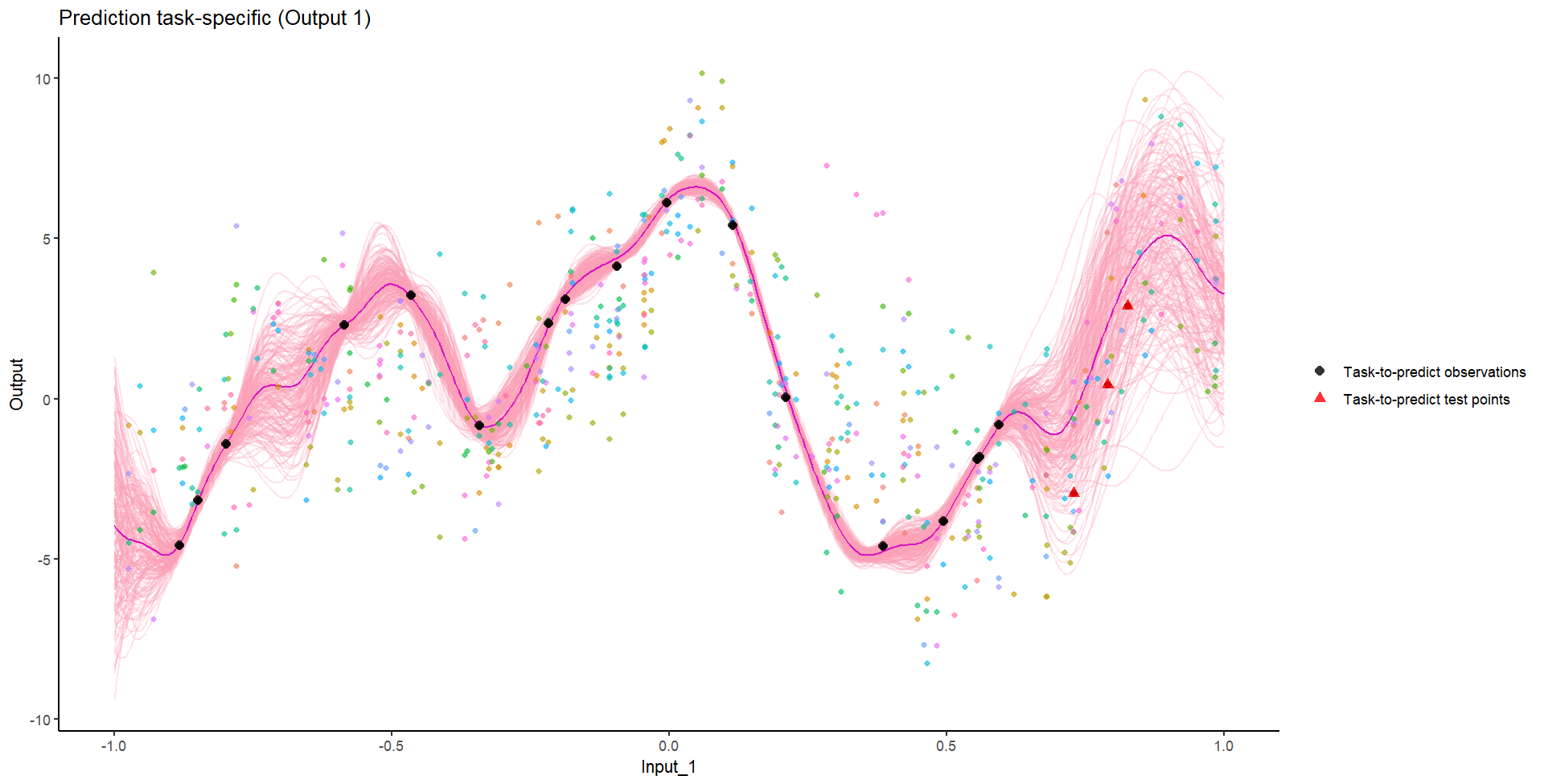
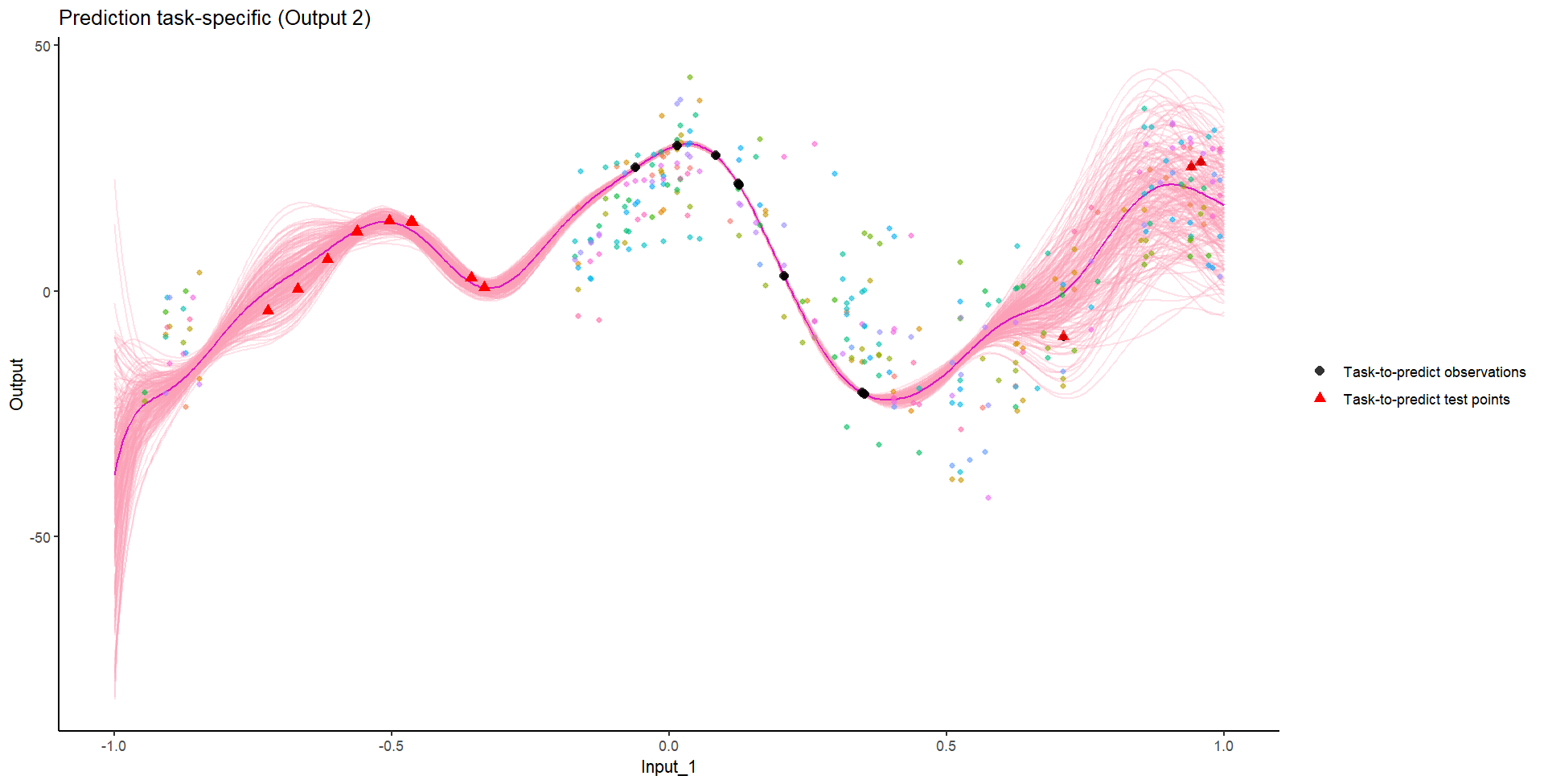
Ok, let’s try something awfully difficult

Let’s remove [-0.8, -0.2] of 2nd Output, and [0.7, 1] of both Outputs for the testing Task.

We don’t even try vanilla GPs, maybe Multi-Output GPs?

• Output 1
• Output 2

Perhaps Multi-Task GPs can do better?

• Output 1
• Output 2

Do we really get the best of both worlds?

• Output 1
• Output 2

Take home messages

• Multi-Output / Multi-task: the same mathematical problem can hide different intuitions on the data and lead to dedicated modelling paradigms,
• Both the mean and covariance parameters can effectively be leveraged to share information,
• Modelling jointly data coming from several sources can costs roughly the same as independant modelling, but can improve dramatically predictive capacities.

Rule of thumb:

Output nature	Framework	Complexity
Independant variables of interest	Single-Task	\(\color{red}{O}\times\mathcal{O}(N^3)\)
Correlated variables of interest	Multi-Output	\(\mathcal{O}(\color{red}{O}^3 N^3)\)
Occurences of the same phenomenon	Multi-Task	\(\mathcal{O}(\color{blue}{T} \times N^3)\)
Occurences of correlated variables	Multi-Task-Multi-Output	\(\mathcal{O}(\color{blue}{T}\times\color{red}{O}^3 N^3)\)

I hope you now \(\mathbb{P}(\text{love Gaussian Processes}) \approx 1\)

Thank you for your attention!





Any questions?