
Apprentissage de données fonctionnelles par modèles multi-tâches :
Application à la prédiction de performances sportives
Arthur Leroy
encadré par
- Servane Gey - MAP5, Université de Paris
- Benjamin Guedj - Inria - University College London
- Pierre Latouche - MAP5, Université de Paris
Soutenance de thèse - 09/12/2020
Origins of the thesis
A problem:
-
Several papers (Boccia & al - 2017, Kearney & Hayes - 2018) point out limits of focusing on best performers in young categories.
-
Sport experts seek new objecive criteria for talent identification.
An opportunity:
-
The French Swimming Federation (FFN) provides a massive database gathering most of the national competition's results since 2002.

Data
Performances in competition for FFN members:
Data
Performances in competition for FFN members:
-
Irregular time series (in number of observations and location),
-
Many different swimmers per category,
Data
Performances in competition for FFN members:
- Irregular time series (in number of observations and location),
- Many different swimmers per category,
- A few observations per swimmer.
Contributions
Are there different patterns of progression among swimmers?
Chapter 2
Leroy et al. - Functional Data Analysis in Sport Science: Example of Swimmers’ Progression Curves Clustering - Applied Sciences - 2018
Can we provide probabilistic predictions of future performances?
Chapter 3
Leroy et al. - Magma: Inference and Prediction with Multi-Task Gaussian Processes - Under submission in Statistics and Computing - https://github.com/ArthurLeroy/MAGMA
May possible group structures improve the quality of predictions?
Chapter 4
Leroy et al. - Cluster-Specific Predictions with Multi-Task Gaussian Processes - Under submission in JMLR - https://github.com/ArthurLeroy/MAGMAclust
Contributions
Are there different patterns of progression among swimmers?
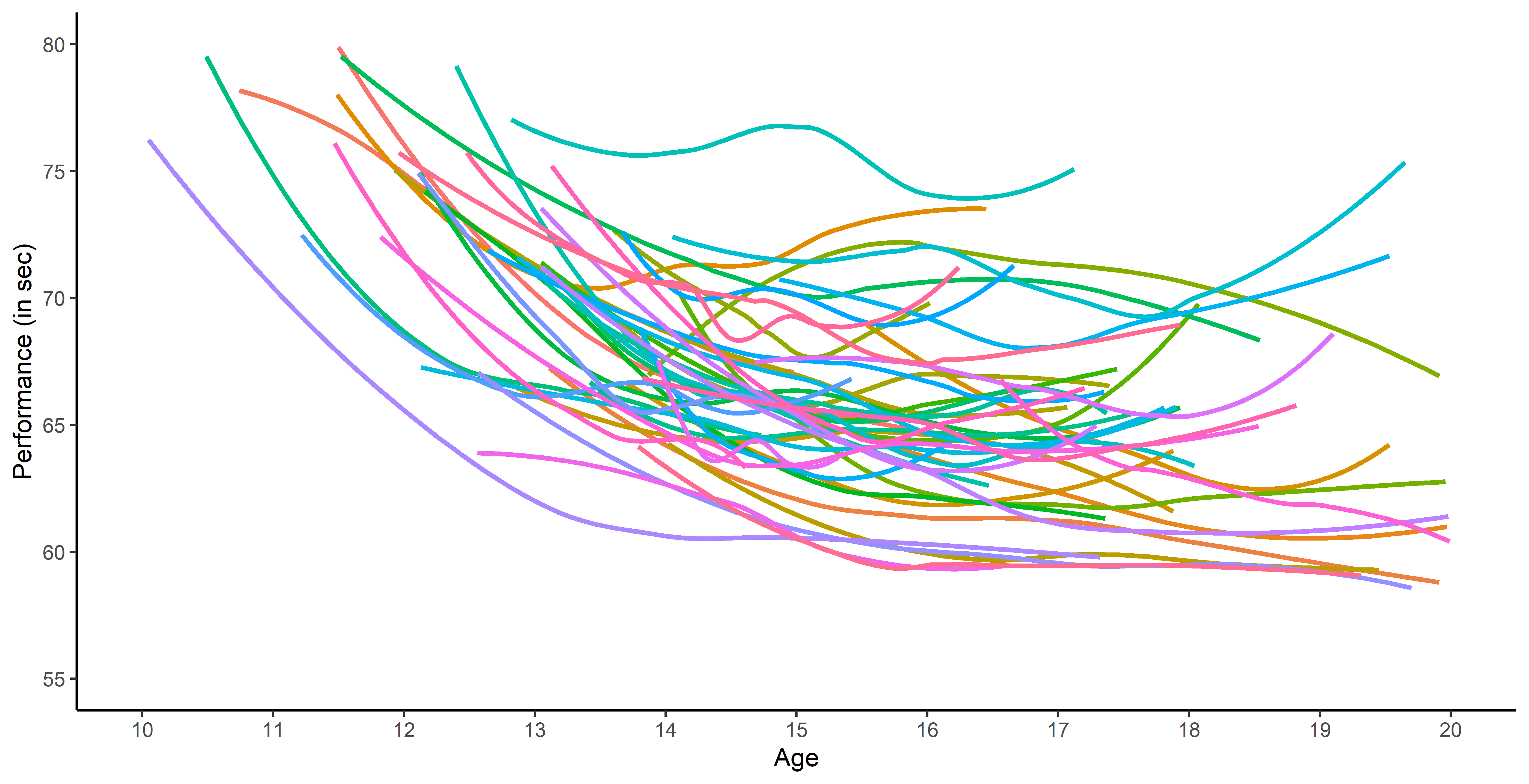
Common representation and curve clustering
A common representation as functional data is proposed by using B-splines decomposition.
Clustering curves with FunHDDC algorithm (Bouveyron & Jacques - 2011, Schmutz et al. - 2020) highlights different patterns of progression. These groups, relating both on level and trend, are consistent groups with sport experts knowledge.
Limits in terms of modelling
This approach suffers from severe limitations such as:
-
unsatisfying individual modellings (side effects, sensibility to sparsity, ...),
-
a lack of probabilistic prediction methods,
-
persisting troubles with irregular measurements.
Contributions
Can we provide probabilistic predictions of future performances?
Gaussian process regression
No restrictions on \(f\) but a prior distribution on a functional space: \(f \sim \mathcal{GP}(0,C(\cdot,\cdot))\)
-
Powerful non parametric method offering probabilistic predictions,
-
Computational complexity in \(\mathcal{O}(N^3)\), with N the number of observations,
-
Correspondence with infinitly wide (deep) neural networks (Neal - 1994, Lee et al. - 2018).
Modelling and prediction with a unique GP
GPs provide an ideal framework for modelling although insufficient for direct predictions.
Multi-task GP with common mean (Magma)
\[y_i = \mu_0 + f_i + \epsilon_i\]
with:
-
\(\mu_0 \sim \mathcal{GP}(m_0, K_{\theta_0}),\)
-
\(f_i \sim \mathcal{GP}(0, \Sigma_{\theta_i}), \ \perp \!\!\! \perp_i,\)
-
\(\epsilon_i \sim \mathcal{GP}(0, \sigma_i^2), \ \perp \!\!\! \perp_i.\)
It follows that:
\[y_i \mid \mu_0 \sim \mathcal{GP}(\mu_0, \Sigma_{\theta_i} + \sigma_i^2 I), \ \perp \!\!\! \perp_i\]
\(\rightarrow\) Unified GP framework with a common mean process \(\mu_0\), and individual-specific process \(f_i\),
\(\rightarrow\) Naturaly handles irregular grids of input data.
Goal: Learn the hyper-parameters, (and \(\mu_0\)'s hyper-posterior).
Difficulty: The likelihood depends on \(\mu_0\), and individuals are not independent.
Notation and dimensionality
Each individual has its specific vector of inputs \(\textbf{t}_i\) associated with outputs \(\textbf{y}_i\).
The mean process \(\mu_0\) requires to define pooled vectors and additional notation follows:
-
\(\textbf{y} = (\textbf{y}_1,\dots, \textbf{y}_i, \dots, \textbf{y}_M)^T,\)
-
\(\textbf{t} = (\textbf{t}_1,\dots,\textbf{t}_i, \dots, \textbf{t}_M)^T,\)
-
\(\textbf{K}_{\theta_0}^{\textbf{t}}\): covariance matrix from the process \(\mu_0\) evaluated on \(\color{red}{\textbf{t}},\)
-
\(\boldsymbol{\Sigma}_{\theta_i}^{\textbf{t}_i}\): covariance matrix from the process \(f_i\) evaluated on \(\color{blue}{\textbf{t}_i},\)
-
\(\Theta = \{ \theta_0, (\theta_i)_i, \sigma_i^2 \}\): the set of hyper-parameters,
-
\(\boldsymbol{\Psi}_{\theta_i, \sigma_i^2}^{\textbf{t}_i} = \boldsymbol{\Sigma}_{\theta_i}^{\textbf{t}_i} + \sigma_i^2 I_{N_i}.\)
While GP are infinite-dimensional objects, a tractable inference on a finite set of observations fully determines the overall properties.
However, handling distributions with differing dimensions constitutes a major technical challenge.
EM algorithm: E step
Assuming to know \(\hat{\Theta}\), the hyper-posterior distribution of \(\mu_0\) is given by: \[
\begin{align}
p(\mu_0(\color{red}{{\mathbf{t}}}) \mid \textbf{y}, \hat{\Theta})
&\propto \mathcal{N}(\mu_0(\color{red}{{\mathbf{t}}}); m_0(\color{red}{\textbf{t}}), \textbf{K}_{\hat{\theta}_0}^{\color{red}{\textbf{t}}}) \times \prod\limits_{i =1}^M \mathcal{N}({\mathbf{y}_i}; \mu_0( \color{blue}{\textbf{t}_i}), \boldsymbol{\Psi}_{\hat{\theta}_i, \hat{\sigma}_i^2}^{\color{blue}{\textbf{t}_i}}) \\
&= \mathcal{N}(\mu_0(\color{red}{{\mathbf{t}}}); \hat{m}_0(\color{red}{\textbf{t}}), \hat{\textbf{K}}^{\color{red}{\textbf{t}}}),
\end{align}
\]
with:
-
\(\hat{\textbf{K}} = \left( {\mathbf{K}_{\hat{\theta}_0}^{\color{red}{\textbf{t}}}}^{-1} + \sum\limits_{i = 1}^M {\boldsymbol{\tilde{\Psi}}_{\hat{\theta}_i \hat{\sigma}_i^2}^{\color{blue}{\textbf{t}_i}}}^{-1} \right)^{-1},\)
-
\(\hat{m}_0(\color{red}{\textbf{t}}) = \hat{\textbf{K}} \left( {\mathbf{K}_{\hat{\theta}_0}^{\color{red}{\textbf{t}}}}^{-1} m_0(\color{red}{\textbf{t}}) + \sum\limits_{i = 1}^M {\boldsymbol{\tilde{\Psi}}_{\hat{\theta}_i, \hat{\sigma}_i^2}^{\color{blue}{\textbf{t}_i}}}^{-1} \tilde{y}_i(\color{blue}{\textbf{t}_i}) \right).\)
EM algorithm: M step
Assuming to know \(p(\mu_0(\color{red}{\textbf{t}}) \mid \textbf{y}, \hat{\Theta})\), the estimated set of hyper-parameters is given by:
\[
\begin{align*}
\hat{\Theta}
&= \underset{\Theta}{\arg\max} \ \mathbb{E}_{\mu_0} [ \log \ p(\textbf{y}, \mu_0(\color{red}{\textbf{t}}) \mid \Theta )] \\
&= \log \mathcal{N} {\left( {\hat{m}_0}(\color{red}{\textbf{t}}); m_0(\color{red}{\textbf{t}}), \mathbf{K}_{\theta_0}^{\color{red}{\textbf{t}}} \right)} - \dfrac{1}{2} Tr {\left( {\hat{\mathbf{K}}}^{\color{red}{\textbf{t}}} {\mathbf{K}_{\theta_0}^{\color{red}{\textbf{t}}}}^{-1} \right)} \\
& \ \ \ + {\sum\limits_{i = 1}^{M}}{\left\{ \log \mathcal{N} {\left( {\mathbf{y}_i}; {\hat{m}_0}(\color{blue}{{\mathbf{t}_i}}), \boldsymbol{\Psi}_{\theta_i, \sigma^2}^{\color{blue}{{\mathbf{t}_i}}} \right)} - \dfrac{1}{2} Tr {\left( {\hat{\mathbf{K}}}^{\color{blue}{{\mathbf{t}_i}}} {\boldsymbol{\Psi}_{\theta_i, \sigma^2}^{\color{blue}{{\mathbf{t}_i}}}}^{-1} \right)} \right\}}.
\end{align*}
\]
EM algorithm: M step
Assuming to know \(p(\mu_0({\mathbf{t}}) \mid \textbf{y}, \hat{\Theta})\), the estimated set of hyper-parameters is given by:
\[
\begin{align*}
\hat{\Theta}
&= \underset{\Theta}{\arg\max} \ \mathbb{E}_{\mu_0} [ \log \ p(\textbf{y}, \mu_0({\mathbf{t}}) \mid \Theta )] \\
&= \log \mathcal{N} {\left( {\hat{m}_0}({\mathbf{t}}); m_0({\mathbf{t}}), \mathbf{K}_{\color{red}{\theta_0}}^{{\mathbf{t}}} \right)} - \dfrac{1}{2} Tr {\left( {\hat{\mathbf{K}}}^{{\mathbf{t}}} {\mathbf{K}_{\color{red}{\theta_0}}^{{\mathbf{t}}}}^{-1} \right)} \\
& \ \ \ + {\sum\limits_{i = 1}^{M}}{\left\{ \log \mathcal{N} {\left( {\mathbf{y}_i}; {\hat{m}_0}({\mathbf{t}_i}), \boldsymbol{\Psi}_{\color{blue}{\theta_i}, \color{blue}{\sigma_i^2}}^{{\mathbf{t}_i}} \right)} - \dfrac{1}{2} Tr {\left( {\hat{\mathbf{K}}}^{{\mathbf{t}_i}} {\boldsymbol{\Psi}_{\color{blue}{\theta_i}, \color{blue}{\sigma_i^2}}^{{\mathbf{t}_i}}}^{-1} \right)} \right\}}.
\end{align*}
\]
-
\({\hat{m}_0}({\mathbf{t}})\) naturally acts like observed values for \(\mu_0\), and \({\hat{\mathbf{K}}}^{{\mathbf{t}}}\) induces a variance penalty term,
-
\(2\) or \(M + 1\) problems of numerical optimisation (analytical gradients are available).
Prediction
For a new individual, we observe some data \(y_*(\textbf{t}_*)\). Let us recall:
\[y_* \mid \mu_0 \sim \mathcal{GP}(\mu_0, \boldsymbol{\Psi}_{\theta_*, \sigma_*^2}), \ \perp \!\!\! \perp_i\]
Goals:
-
derive a analytical predictive distribution at arbitrary inputs \({\mathbf{t}^{p}}\),
-
sharing the information from training individuals, stored in the mean process \(\mu_0\).
Difficulties:
-
the model is conditionned over \(\mu_0\), a latent, unobserved quantity,
-
defining the adequate target distribution is not straightforward,
-
working on a new grid of inputs \({\mathbf{t}^{p}_{*}}= ({\mathbf{t}_{*}}, {\mathbf{t}^{p}})^{\intercal},\) potentially distinct from \({\mathbf{t}}.\)
Prediction: the key idea
Defining a multi-task prior distribution by:
-
conditioning on training data,
-
integrating over \(\mu_0\)'s hyper-posterior distribution.
\[\begin{align}
p(y_* (\textbf{t}_*^{p}) \mid \textbf{y})
&= \int p\left(y_* (\textbf{t}_*^{p}) \mid \textbf{y}, \mu_0(\textbf{t}_*^{p})\right) p(\mu_0 (\textbf{t}_*^{p}) \mid \textbf{y}) \ d \mu_0({\mathbf{t}^{p}_{*}}) \\
&= \int \underbrace{ p \left(y_* (\textbf{t}_*^{p}) \mid \mu_0 (\textbf{t}_*^{p}) \right)}_{\mathcal{N}(y_*; \mu_0, \Psi_*)} \ \underbrace{p(\mu_0 (\textbf{t}_*^{p}) \mid \textbf{y})}_{\mathcal{N}(\mu_0; \hat{m}_0, \hat{K})} \ d \mu_0({\mathbf{t}^{p}_{*}}) \\
&= \mathcal{N}( \hat{m}_0 ({\mathbf{t}^{p}_{*}}), \Gamma)
\end{align}\]
with:
\[\Gamma = \boldsymbol{\Psi}_{\theta_*, \sigma_*^2}^{{\mathbf{t}^{p}_{*}}} + \hat{K}^{{\mathbf{t}^{p}_{*}}}\]
Prediction: additional steps
-
Multi-task prior:
\[p {\left( \begin{bmatrix}
y_*(\color{red}{{\mathbf{t}_{*}}}) \\
y_*(\color{blue}{{\mathbf{t}^{p}}}) \\
\end{bmatrix} \mid \textbf{y} \right)} = \mathcal{N} {\left(
\begin{bmatrix}
y_*(\color{red}{{\mathbf{t}_{*}}}) \\
y_*(\color{blue}{{\mathbf{t}^{p}}}) \\
\end{bmatrix}; \
\begin{bmatrix}
\hat{m}_0(\color{red}{{\mathbf{t}_{*}}}) \\
\hat{m}_0(\color{blue}{{\mathbf{t}^{p}}}) \\
\end{bmatrix},
\begin{pmatrix}
\Gamma_{\color{red}{**}} & \Gamma_{\color{red}{*}\color{blue}{p}} \\
\Gamma_{\color{blue}{p}\color{red}{*}} & \Gamma_{\color{blue}{pp}}
\end{pmatrix} \right)}\]
-
Multi-task posterior:
\[p(y_*(\color{blue}{{\mathbf{t}^{p}}}) \mid y_*(\color{red}{{\mathbf{t}_{*}}}), \textbf{y}) = \mathcal{N} \Big( y_*(\color{blue}{{\mathbf{t}^{p}}}); \ \hat{\mu}_{*}(\color{blue}{{\mathbf{t}^{p}}}) , \hat{\Gamma}_{\color{blue}{pp}} \Big)\]
with:
-
\(\hat{\mu}_{*}(\color{blue}{{\mathbf{t}^{p}}}) = \hat{m}_0(\color{blue}{{\mathbf{t}^{p}}}) + \Gamma_{\color{blue}{p}\color{red}{*}}\Gamma_{\color{red}{**}}^{-1} (y_*(\color{red}{{\mathbf{t}_{*}}}) - \hat{m}_0 (\color{red}{{\mathbf{t}_{*}}}))\)
-
\(\hat{\Gamma}_{\color{blue}{pp}} = \Gamma_{\color{blue}{pp}} - \Gamma_{\color{blue}{p}\color{red}{*}}\Gamma_{\color{red}{**}}^{-1} \Gamma_{\color{red}{*}\color{blue}{p}}\)
This multi-task posterior distribution provides the desired probabilistic predictions.
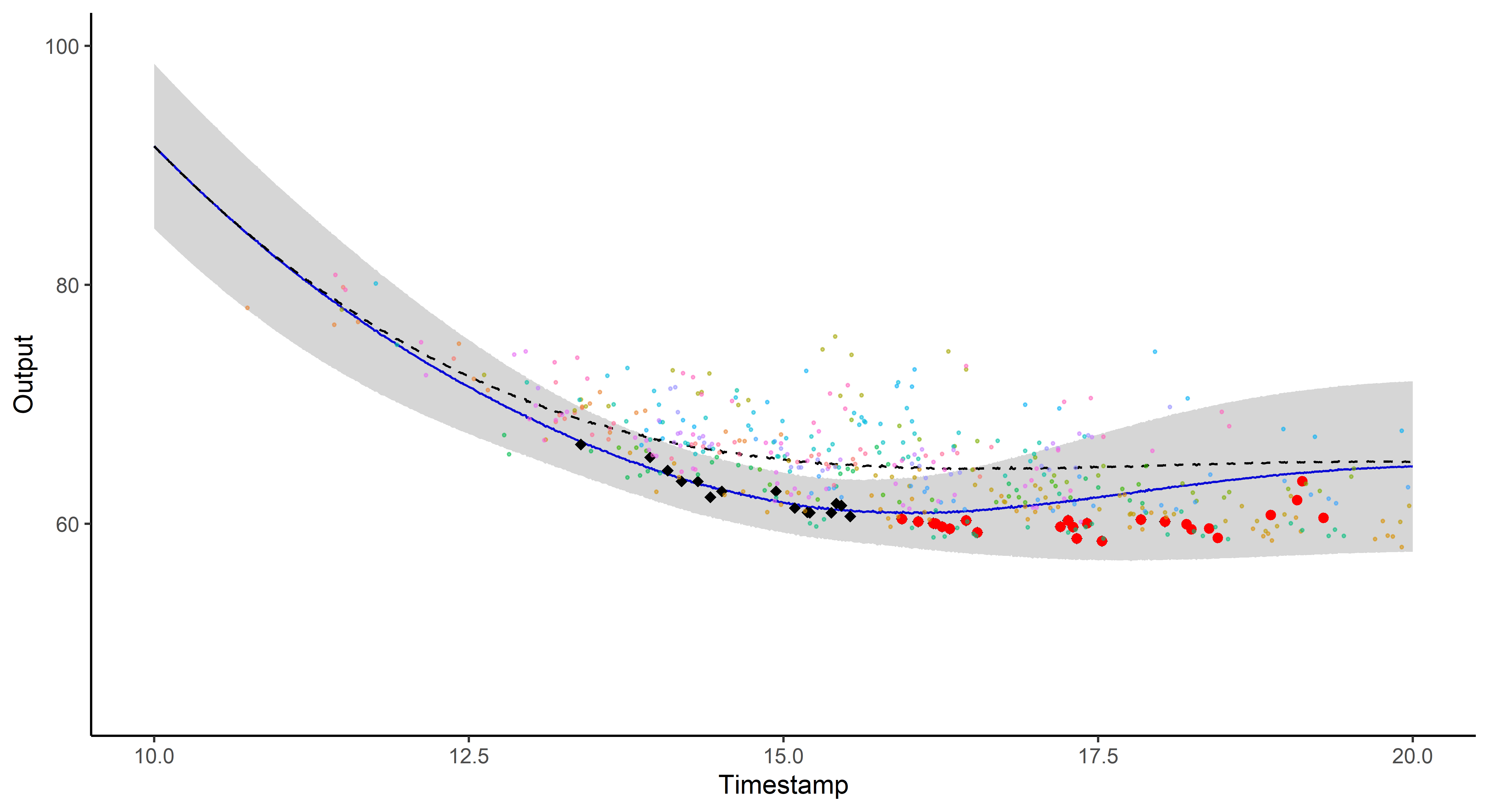
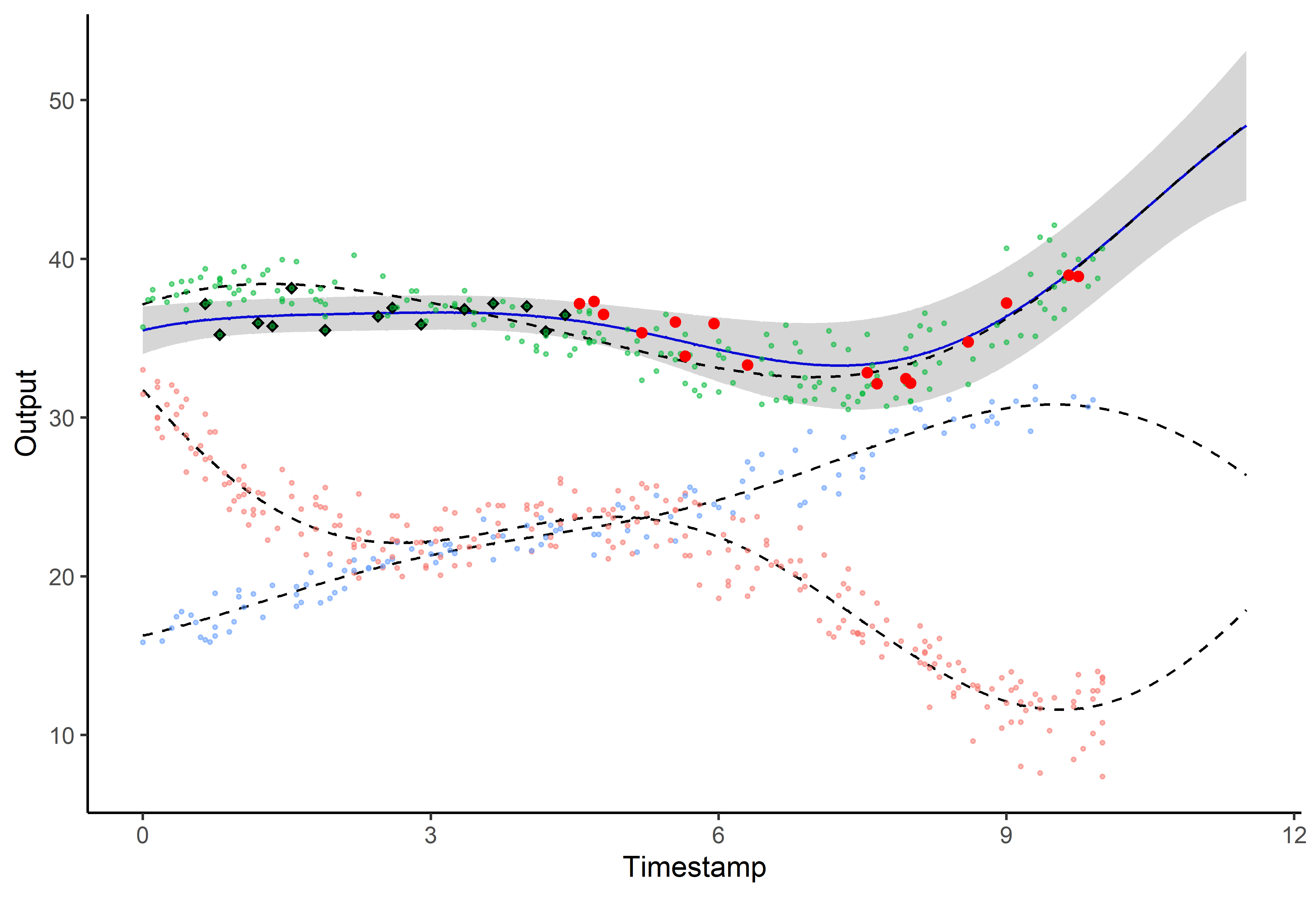
A picture is worth 1000 words
- Same data, same hyper-parameters
- Standard GP (left), Magma (right)
A GIF is worth \(10^9\) words
Illustration: GP regression
Contributions
May eventual group structures improve the quality of predictions?
Magma + Clustering = MagmaClust
A unique underlying mean process might be too restrictive.
\(\rightarrow\) Mixture of multi-task GPs:
\[y_i = \mu_0 + f_i + \epsilon_i\]
with:
-
\(\color{red}{Z_{i}} \sim \mathcal{M}(1, \color{red}{\boldsymbol{\pi}}), \ \perp \!\!\! \perp_i,\)
- \(\mu_0 \sim \mathcal{GP}(m_0, K_{\theta_0}), \ \perp \!\!\! \perp_k,\)
- \(f_i \sim \mathcal{GP}(0, \Sigma_{\theta_i}), \ \perp \!\!\! \perp_i,\)
- \(\epsilon_i \sim \mathcal{GP}(0, \sigma_i^2), \ \perp \!\!\! \perp_i.\)
It follows that:
\[y_i \mid \mu_0 \sim \mathcal{GP}(\mu_0, \Sigma_{\theta_i} + \sigma_i^2 I), \ \perp \!\!\! \perp_i\]
Magma + Clustering = MagmaClust
A unique underlying mean process might be too restrictive.
\(\rightarrow\) Mixture of multi-task GPs:
\[y_i \mid \{\color{red}{Z_{ik}} = 1 \} = \mu_{\color{red}{k}} + f_i + \epsilon_i\]
with:
- \(\color{red}{Z_{i}} \sim \mathcal{M}(1, \color{red}{\boldsymbol{\pi}}), \ \perp \!\!\! \perp_i,\)
- \(\mu_{\color{red}{k}} \sim \mathcal{GP}(m_{\color{red}{k}}, \color{red}{C_{\gamma_{k}}})\ \perp \!\!\! \perp_{\color{red}{k}},\)
- \(f_i \sim \mathcal{GP}(0, \Sigma_{\theta_i}), \ \perp \!\!\! \perp_i,\)
- \(\epsilon_i \sim \mathcal{GP}(0, \sigma_i^2), \ \perp \!\!\! \perp_i.\)
It follows that:
\[y_i \mid \{ { \boldsymbol{\mu} }, \color{red}{\boldsymbol{\pi}} \} \sim \sum\limits_{k=1}^K{ \color{red}{\pi_k} \ \mathcal{GP}\Big(\mu_{\color{red}{k}}, \Psi_i \Big)}, \ \perp \!\!\! \perp_i\]
Learning
The integrated likelihood is not tractable anymore due to posterior dependencies between \({ \boldsymbol{\mu} }= \{\mu_k\}_k\) and \({\mathbf{Z}}= \{Z_i\}_i\).
Variational inference still allows us to maintain closed-form approximations. For any distribution \(q\): \[\log p(\textbf{y} \mid \Theta) = \mathcal{L}(q; \Theta) + KL \big( q \mid \mid p(\boldsymbol{\mu}, \boldsymbol{Z} \mid \textbf{y}, \Theta)\big)\]
The posterior independance is forced by an approximation assumption: \(q(\boldsymbol{\mu}, \boldsymbol{Z}) = q_{\boldsymbol{\mu}}(\boldsymbol{\mu})q_{\boldsymbol{Z}}(\boldsymbol{Z}).\)
Maximising the lower bound \(\mathcal{L}(q; \Theta)\) induces natural factorisations over clusters and individuals for the variational distributions.
Variational EM: E step
The optimal variational distributions are analytical and factorise such as:
\[
\begin{align}
\hat{q}_{\boldsymbol{\mu}}(\boldsymbol{\mu}) &= \prod\limits_{k = 1}^K \mathcal{N}(\mu_k;\hat{m}_k, \hat{\textbf{C}}_k) \\
\hat{q}_{\boldsymbol{Z}}(\boldsymbol{Z}) &= \prod\limits_{i = 1}^M \mathcal{M}(Z_i;1, \color{red}{\boldsymbol{\tau}_i})
\end{align}
\]
with:
\[
\color{red}{{\tau_{ik}}} = \dfrac{{\hat{\pi}_{k}}\ {\mathcal{N}}{\left( {\mathbf{y}_i}; {\hat{m}_k}, {\boldsymbol{\Psi}_{\hat{\theta}_i, \hat{\sigma}_i^2}}\right)} \exp {\left( -\frac{1}{2} {\textrm{tr}\left( {{\boldsymbol{\Psi}_{\hat{\theta}_i, \hat{\sigma}_i^2}}}^{-1} \hat{\textbf{C}}_k \right)} \right)} }{\sum\limits_{l = 1}^{K} {\hat{\pi}_{l}}\ {\mathcal{N}}{\left( {\mathbf{y}_i}; \hat{m}_l , {\boldsymbol{\Psi}_{\hat{\theta}_i, \hat{\sigma}_i^2}}\right)} \exp{\left( -\frac{1}{2} {\textrm{tr}\left( {{\boldsymbol{\Psi}_{\hat{\theta}_i, \hat{\sigma}_i^2}}}^{-1} \hat{\textbf{C}}_l \right)} \right)}}, \ \forall i, \forall k.
\]
Variational EM: M step
Optimising \(\mathcal{L}(\hat{q}; \Theta)\) w.r.t. \(\Theta\) induces independant maximisation problems:
\[
\begin{align*}
\hat{\Theta}
&= \text{arg}\max\limits_{\Theta} \mathbb{E}_{\boldsymbol{\mu},\boldsymbol{Z}} \left[ \log p(\textbf{y},\boldsymbol{\mu}, \boldsymbol{Z} \mid \Theta)\right] \\
&= {\sum\limits_{k = 1}^{K}}\ \mathcal{N} {\left( {\hat{m}_k}; \ m_k, \boldsymbol{C}_{\color{red}{\gamma_k}} \right)} - \dfrac{1}{2} {\textrm{tr}\left( {\mathbf{\hat{C}}_k}\boldsymbol{C}_{\color{red}{\gamma_k}}^{-1}\right)} \\
& \hspace{1cm} + {\sum\limits_{k = 1}^{K}}{\sum\limits_{i = 1}^{M}}{\tau_{ik}}\ \mathcal{N} {\left( {\mathbf{y}_i}; \ {\hat{m}_k}, \boldsymbol{\Psi}_{\color{blue}{\theta_i}, \color{blue}{\sigma_i^2}} \right)} - \dfrac{1}{2} {\textrm{tr}\left( {\mathbf{\hat{C}}_k}\boldsymbol{\Psi}_{\color{blue}{\theta_i}, \color{blue}{\sigma_i^2}}^{-1}\right)} \\
& \hspace{1cm} + {\sum\limits_{k = 1}^{K}}{\sum\limits_{i = 1}^{M}}{\tau_{ik}}\log \color{green}{{\pi_{k}}}
\end{align*}
\]
Covariance structure assumption: 4 sub-models
Sharing the covariance structures offers a compromise between flexibility and parsimony:
-
\(\mathcal{H}_{oo}:\) common mean process - common individual process - \(\color{orange}{2}\) HPs,
-
\(\mathcal{H}_{\color{red}{k}o}:\) specific mean process - common individual process - \(\color{orange}{K + 1}\) HPs,
-
\(\mathcal{H}_{o\color{blue}{i}}:\) common mean process - specific individual process - \(\color{orange}{M + 1}\) HPs,
-
\(\mathcal{H}_{\color{red}{k}\color{blue}{i}}:\) specific mean process - specific individual process - \(\color{orange}{M + K}\) HP.
Prediction
-
EM for estimating \(p(\color{red}{Z_*} \mid \textbf{y}, \hat{\Theta})\), \(\hat{\theta}_*\), and \(\hat{\sigma}_*^2\),
-
Multi-task prior: \[
p {\left( \begin{bmatrix}
y_*(\textbf{t}_*) \\
y_*(\textbf{t}_p) \\
\end{bmatrix} \mid \color{red}{Z_{*k}}=1 , \textbf{y} \right)} = \mathcal{N} {\left( \begin{bmatrix}
y_*(\textbf{t}_*) \\
y_*(\textbf{t}_p) \\
\end{bmatrix};
\begin{bmatrix}
\hat{m}_k(\textbf{t}_*) \\
\hat{m}_k(\textbf{t}^p) \\
\end{bmatrix},
\begin{pmatrix}
\Gamma_{**}^k & \Gamma_{*p}^k \\
\Gamma_{p*}^k & \Gamma_{pp}^k
\end{pmatrix} \right)}, \color{red}{\forall k},
\]
-
Multi-task posterior:
\[
p(y_*(\textbf{t}^p) \mid y_*(\textbf{t}_*), \color{red}{Z_{*k}} = 1, \textbf{y}) = \mathcal{N} \big( \hat{\mu}_{*}^k (\textbf{t}^p) , \hat{\Gamma}_{pp}^{k} \big), \ \color{red}{\forall k},
\]
-
Predictive multi-task GPs mixture:
\[p(y_*(\textbf{t}^p) \mid y_*(\textbf{t}_*), \textbf{y}) = \color{red}{\sum\limits_{k = 1}^{K} \tau_{*k}} \ \mathcal{N} \big( \hat{\mu}_{*}^k(\textbf{t}^p) , \hat{\Gamma}_{pp}^k(\textbf{t}^p) \big).\]
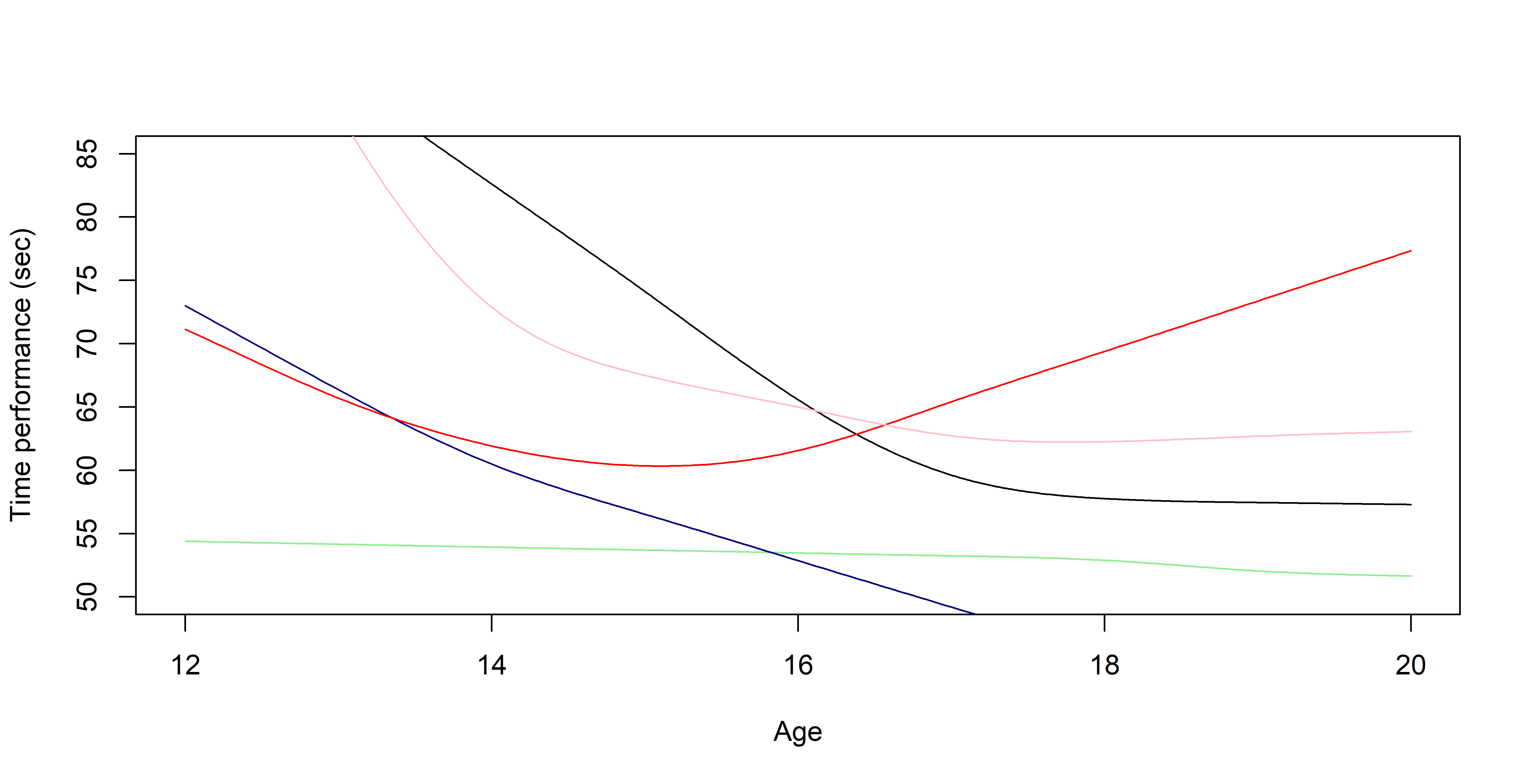
Illustration: Magma vs MagmaClust
And what about the swimmers ?
Standard GP regression
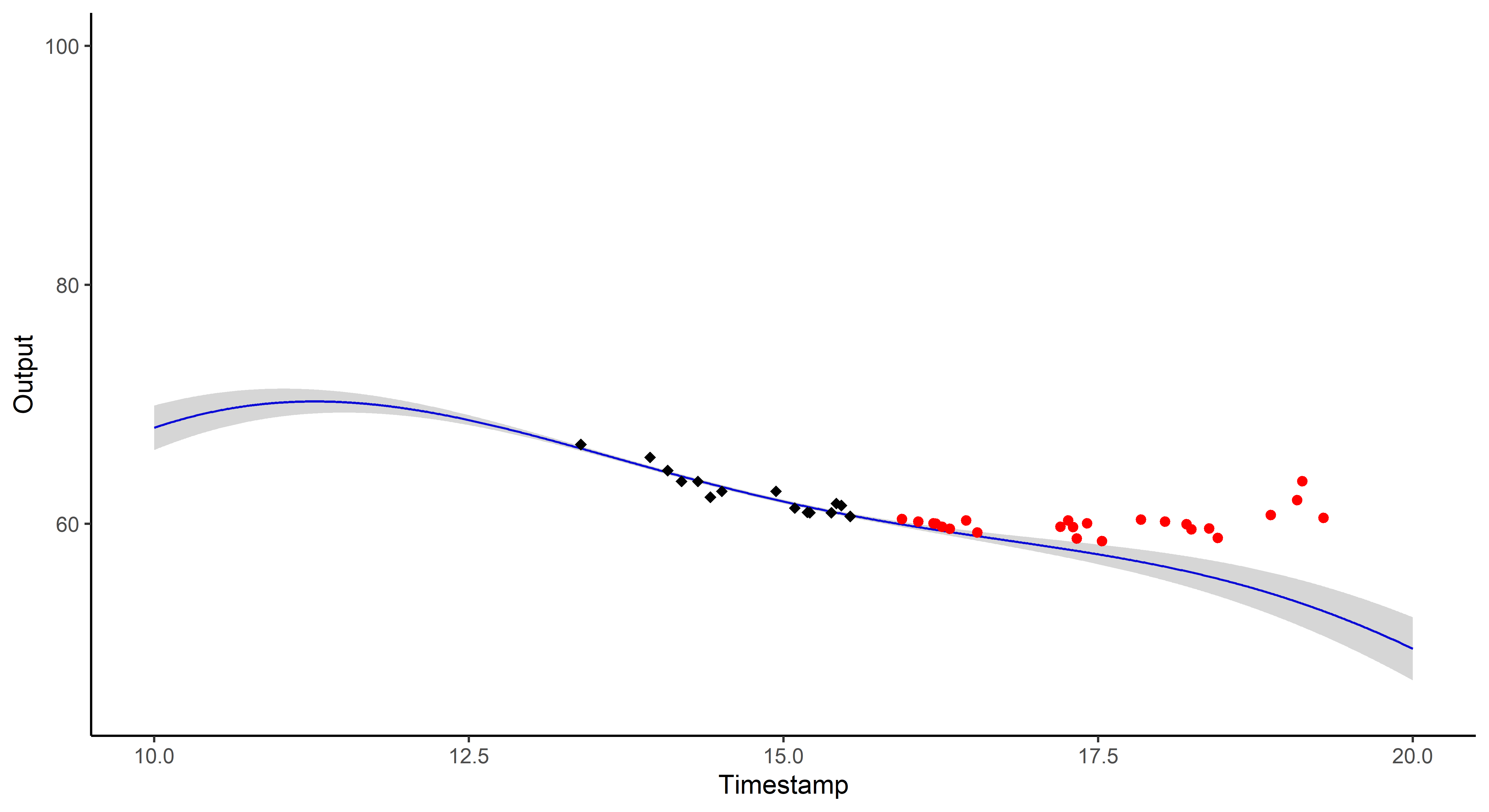
And what about the swimmers ?
Magma
And what about the swimmers ?
MagmaClust
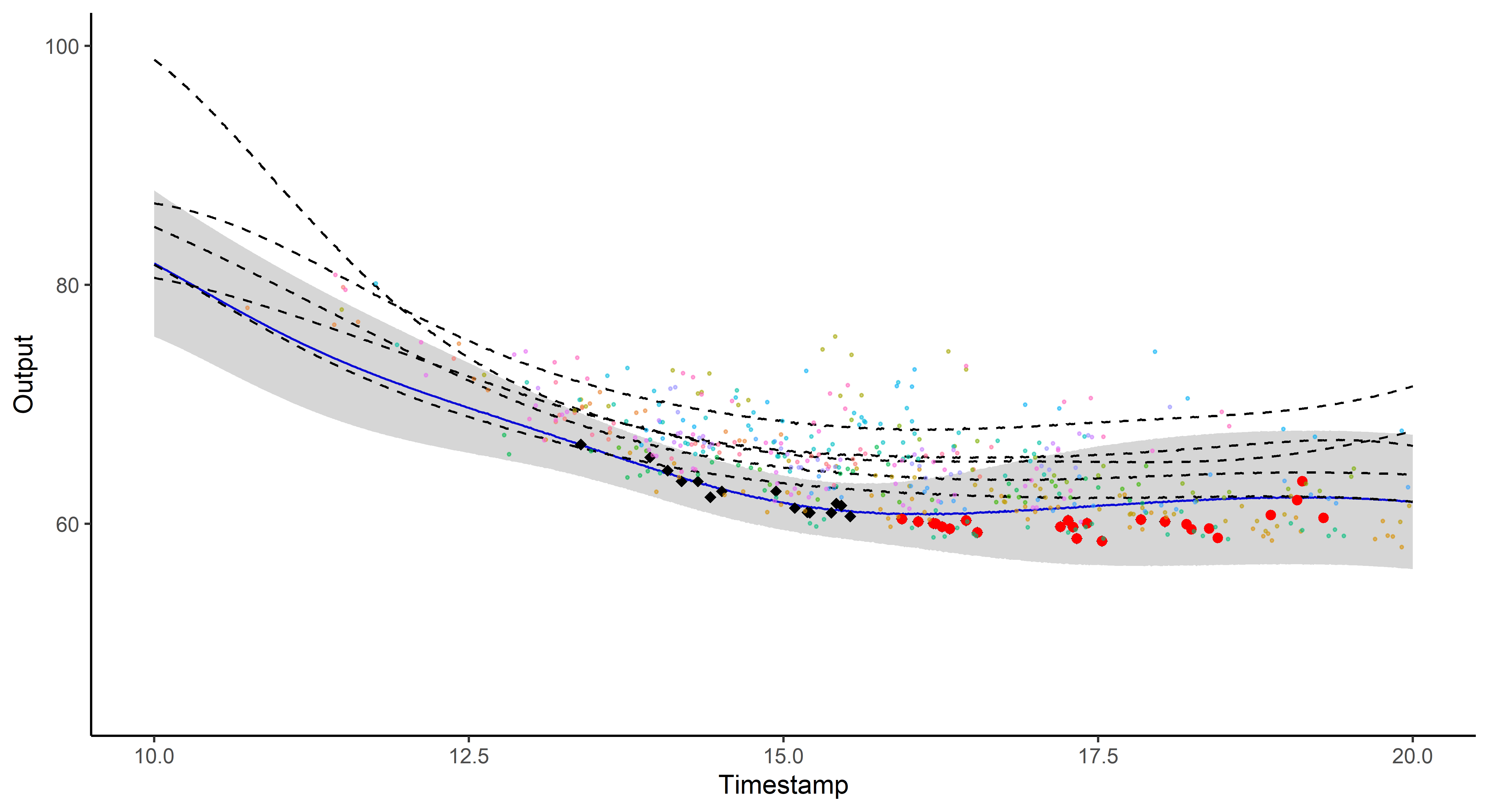
Did I mention that I like GIFs ?
Perspectives: model selection in MagmaClust
Leroy & al. - 2020 - preprint
After convergence of the VEM algorithm, a variational-BIC expression can be derived as:
\[\begin{align*}
VBIC(K)
&= \mathcal{L}(\hat{q}; \hat{\Theta}) - \dfrac{\mathrm{card}\{HP \}}{2} \log M \\
&= \sum\limits_{i=1}^M \sum\limits_{k=1}^K \left[ \tau_{ik} \left( \log \mathcal{N}\left( \mathbf{y}_i; \hat{m}_k(\mathbf{t}_i), {\boldsymbol{\Psi}_{\hat{\theta}_i, \hat{\sigma}_i^2}^{\mathbf{t}_i}} \right) - \dfrac{1}{2} Tr ( \mathbf{\hat{C}}_k^{\mathbf{t}} {\boldsymbol{\Psi}_{\hat{\theta}_i, \hat{\sigma}_i^2}^{\mathbf{t}_i}}^{-1}) + \log \dfrac{\hat{\pi_k}}{\tau_{ik}} \right) \right] \\
& \hspace{0.5cm} + \sum\limits_{k=1}^K \Bigg[ \log \mathcal{N} \left( \hat{m}_k(\textbf{t}); m_k(\mathbf{t}) , {\mathbf{C}_{\hat{\gamma}_k}^{\mathbf{t}^{p}_{*}}} \right) - \dfrac{1}{2} Tr( \mathbf{\hat{C}}_k^{\mathbf{t}} {\mathbf{C}_{\hat{\gamma}_k}^{\mathbf{t}^{p}_{*}}}^{-1}) \\
& \hspace{2cm} + \dfrac{1}{2} \log \mid \mathbf{\hat{C}}_k^{\mathbf{t}} \mid + N \log 2 \pi + N \Bigg] - \dfrac{\alpha_i + \alpha_k + (K - 1)}{2} \log M.
\end{align*}\]
Perspectives
-
Enable association with sparse GP approximations,
-
Extend to multivariate functional regression,
-
Develop an online version,
-
Integrate to the FFN app and launch real-life tests,
-
Investigate GP variational encoder for functional data
Thank you for your attention
References
- Neal - Priors for infinite networks - University of Toronto - 1994
- Shi and Wang - Curve prediction and clustering with mixtures of Gaussian process functional regression models - Statistics and Computing - 2008
- Bouveyron and Jacques - Model-based clustering of time series in group-specific functional subspaces - Advances in Data Analysis and Classification - 2011
- Boccia et al. - Career Performance Trajectories in Track and Field Jumping Events from Youth to Senior Success: The Importance of Learning and Development - PLoS ONE - 2017
- Lee et al. - Deep Neural Networks as Gaussian Processes - ICLR - 2018
- Kearney et Hayes - Excelling at youth level in competitive track and field athletics is not a prerequisite for later success - Journal of Sports Sciences - 2018
- Leroy et al. - Functional Data Analysis in Sport Science: Example of Swimmers’ Progression Curves Clustering - Applied Sciences - 2018
- Schmutz et al. - Clustering multivariate functional data in group-specific functional subspaces - Computational Statistics - 2020
- Leroy et al. - Magma: Inference and Prediction with Multi-Task Gaussian Processes - Under review - 2020
- Leroy et al. - Cluster-Specific Predictions with Multi-Task Gaussian Processes - Under review - 2020
Annexe
Two important prediction steps of Magma have been omitted for clarity:
- Recomputing the hyper-posterior distribution on the new grid: \[
p{\left( \mu_0 (\textbf{t}_*^{p}) \mid \textbf{y} \right)},
\]
- Estimating the hyper-parameters of the new individual: \[
\hat{\theta}_*, \hat{\sigma}_*^2 = \underset{\theta_*, \sigma_*^2}{\arg\max} \ p(y_* (\textbf{t}_*) \mid \textbf{y}, \theta_*, \sigma_*^2 ).
\]
The computational complexity for learning is given by:
- Magma: \[
\mathcal{O}(M\times N_i^3 + N^3)
\]
- MagmaClust: \[
\mathcal{O}(M\times N_i^3 + K \times N^3)
\]
Annexe: MagmaClust, remaining clusters