Apprentissage de données fonctionnelles par modèles multi-tâches :
Application à la prédiction de performances sportives

Context

Traditional talent identification: \(\rightarrow\) Best young athlete + coach intuition

G. Boccia et al. (2017) :

\(\simeq\) 60% of 16 years old elite athletes do not maintain their level of performance

Philip E. Kearney & Philip R. Hayes (2018) :

\(\simeq\) only 10% of senior top 20 were also top 20 before 13 years

Data

Performances from FF of Swimming members since 2002:

• Irregular time series
• Different number \(N_i\) of observations between individuals
• Different observational timestamps \(t_i^k\)
• \(N_i\) \(\simeq x \times10^1\)

Data

Performances from FF of Swimming members since 2002:

• Irregular time series
• Different number \(N_i\) of observations between individuals
• Different observational timestamps \(t_i^k\)
• \(N_i\) \(\simeq x \times10^1\) | \(N\) \(= \sum\limits_{i=1}^{M}\) \(N_i\) \(\simeq x \times 10^5\)

Data

Performances from FF of Swimming members since 2002:

• Irregular time series
• Different number \(N_i\) of observations between individuals
• Different observational timestamps \(t_i^k\)
• \(N_i\) \(\simeq x \times10^1\) | \(N\) \(= \sum\limits_{i=1}^{M}\) \(N_i\) \(\simeq x \times 10^5\)

Curves clustering

Functional data \(\simeq\) coefficients \(\alpha_k\) of B-splines functions:

\[y_i(t) = \sum\limits_{k=1}^{K}{\alpha_k B_k(t)}\]

Clustering: Algo FunHDDC (Gaussian mixture + EM) Bouveyron & Jacques - 2011

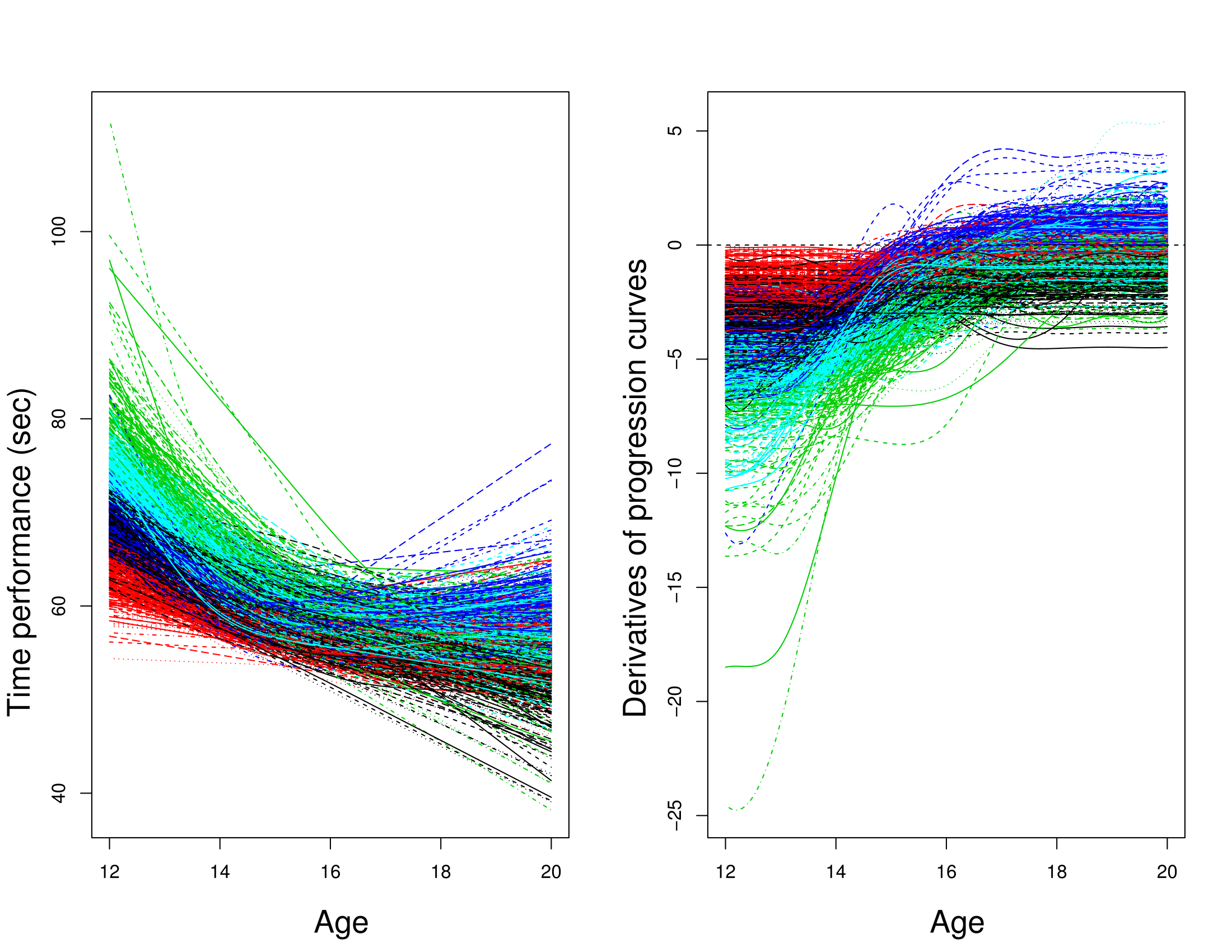
Using the multidimensional version : curve + derivative \(\rightarrow\) Information about performance level and trend of improvement

Curve clustering

Leroy et al. - 2018

• Different patterns of progression
• Consistent groups for sports experts

Curve clustering

Leroy et al. - 2018

• Different patterns of progression
• Consistent groups for sport experts

New objectives

• Prediction of the future values of the progression curve \(\rightarrow\) Functional regression
• Quantification of prediction uncertainty \(\rightarrow\) Probabilistic framework

Gaussian process regression

Bishop - 2006 | Rasmussen & Williams - 2006

GPR : a kernel method to estimate \(f\) when:

\[y = f(x) +\epsilon\]

\(\rightarrow\) No restrictions on \(f\) but a prior probability:

\[f \sim \mathcal{GP}(0,C(\cdot,\cdot))\]

An example of exponential kernel for the covariance function: \[cov(f(x),f(x'))= C(x,x') = \alpha exp(- \dfrac{1}{2\theta^2} |x - x'|^2)\] Kernel definition \(\Rightarrow\) prefered properties on \(f\)

Prediction

\(\textbf{y}_{N+1} = (y_1,...,y_{N+1})\) has the following prior density: \[\textbf{y}_{N+1} \sim \mathcal{N}(0, C_{N+1}), \ C_{N+1} = \begin{pmatrix} C_N & k_{N+1} \\ k_{N+1}^T & c_{N+1} \end{pmatrix}\]

When the joint density is gaussian, so does the conditionnal dentisty:

\[y_{N+1}|\textbf{y}_{N}, \textbf{x}_{N+1} \sim \mathcal{N}(k^T \color{red}{C_N^{-1}}\textbf{y}_{N}, c_{N+1}- k_{N+1}^T \color{red}{C_N^{-1}} k_{N+1})\]

• Prediction: \(\hat{y}_{N+1} = \mathbb{E}[y_{N+1}|\textbf{y}_{N}, \textbf{x}_{N+1}]\)
• Uncertainty: CI with \(\mathbb{V}[y_{N+1}|\textbf{y}_{N}, \textbf{x}_{N+1}]\)

Visualization of GPR

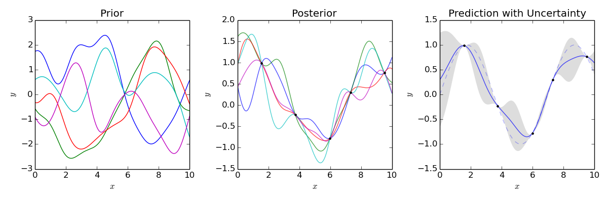
Key points:

• Define a covariance function with desirable properties
• Non parametric method giving probabilistic predictions
• Complexity \(O(\color{red}{N^3})\) (inversion of an \(\color{red}{N} \times \color{red}{N}\) matrix)

GP estimation from data

Estimating a GP on each individual (\(O(\color{green}{N_i^3})\)):

• Uncertainty: Ok

GP estimation from data

Estimating a GP on each individuals (\(O(\color{green}{N_i^3})\)):

• Uncertainty: Ok

GP estimation from data

Estimating a GP on each individuals (\(O(\color{green}{N_i^3})\)):

• Uncertainty: Ok

GP estimation from data

Estimating a GP on each individuals (\(O(\color{green}{N_i^3})\)):

• Uncertainty: Ok

GP estimation from data

Estimating a GP on each individuals (\(O(\color{green}{N_i^3})\)):

• Uncertainty: Ok

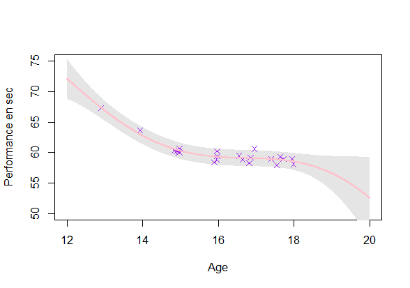
Reaching a coherent modeling

Estimating a GP on each individuals (\(O(\color{green}{N_i^3})\)):

• Uncertainty: Ok
• Coherence: Improvement required

\(\rightarrow\) Using the shared information between individuals (GPR-ME)

The GPFR model

Shi & Wang - 2008 | Shi & Choi - 2011

\[y_i(t) = \mu_0(t) + f_i(t) + \epsilon_i\] with:

• \(\mu_0(t) = \sum\limits_{k =1}^{K} \alpha_k \mathcal{B}_k(t)\) with \((\mathcal{B}_k)_k\) a spline basis
• \(f_i(\cdot) \sim \mathcal{GP}(0, \Sigma_{\theta_i}(\cdot,\cdot)), \ f_i \perp \!\!\! \perp\)
• \(\epsilon_i \sim \mathcal{N}(0, \sigma_i^2), \ \epsilon_i \perp \!\!\! \perp\)

GPFDA R package

Limits:

• No uncertainty about \(\mu_0\)
• Does not allow irregular time series

Multi-task Gaussian processes with common mean (MAGMA)

\[y_i(t) = \mu_0(t) + f_i(t) + \epsilon_i\] with:

• \(\mu_0(\cdot) \sim \mathcal{GP}(m_0(\cdot), K_{\theta_0}(\cdot,\cdot))\)
• \(f_i(\cdot) \sim \mathcal{GP}(0, \Sigma_{\theta_i}(\cdot,\cdot)), \ f_i \perp \!\!\! \perp\)
• \(\epsilon_i \sim \mathcal{N}(0, \sigma_i^2), \ \epsilon_i \perp \!\!\! \perp\)

It follows that:

\[y_i(\cdot) \vert \mu_0 \sim \mathcal{GP}(\mu_0(\cdot), \Sigma_{\theta_i}(\cdot,\cdot) + \sigma_i^2), \ y_i \vert \mu_0 \perp \!\!\! \perp\]

\(\rightarrow\) Shared information through \(\mu_0\) and its uncertainty \(\rightarrow\) Unified non parametric probabilistic framework \(\rightarrow\) Effective even for irregular time series

Notations

\(\textbf{y} = (y_1^1,\dots,y_i^k,\dots,y_M^{N_M})^T\) \(\textbf{t} = (t_1^1,\dots,t_i^k,\dots,t_M^{N_M})^T\) \(\Theta = \{ \theta_0, (\theta_i)_i, \sigma_i^2 \}\)

\(K\): covariance matrix from the process \(\mu_0\) evaluated on \(\textbf{t}\)

\(K = \left[ K_{\theta_0}(t_i^k, t_j^l) \right]_{(i,j), (k,l)}\)

\(\Sigma_i\): covariance matrix from the process \(f_i\) evaluated on \(\textbf{t}_i\)

\(\Sigma_i = \left[ \Sigma_{\theta_i}(t_i^k, t_i^l) \right]_{(k,l)} \ \ \forall i = 1, \dots, M\)

\(\Psi_i = \Sigma_i + \sigma_i^2 I_{N_i}\)

Bayes' law is the new black

Reminder of its simple definition:

\[ \mathbb{P}(T \vert D) = \dfrac{\mathbb{P}(D \vert T) \mathbb{P}(T)}{\mathbb{P}(D)} \] Powerful implication when it comes to learning from data:

• \(\mathbb{P}(T)\), probability of your theory, what you think a priori
• \(\mathbb{P}(D \vert T)\), probability of data if theory is true, likelihood
• \(\mathbb{P}(D)\), probability that your data occur, norm. constant

Bayes' law tells you how and what you should learn on theory T according to data D:

\(\rightarrow \mathbb{P}(T \vert D)\), what you should think a posteriori Computational burden, among solutions: empirical Bayes

Learning HPs and \(\mu_0\) : an EM algorithm

Step E: Computing the posterior (knowing \(\Theta\))

\[ \begin{align} p(\mu_0(\textbf{t}) \vert \textbf{t}, \textbf{y}, \Theta) &\propto p(\textbf{y} \vert \textbf{t}, \mu_0(\textbf{t}), \Theta) \ p(\mu_0(\textbf{t}) \vert \textbf{t}, \Theta) \\ &\propto \prod\limits_{i =1}^M \mathcal{N}( \mu_0(\textbf{t}_i), \Psi_i) \ \mathcal{N}(m_0(\textbf{t}), K) \\ &= [Insert \ here \ some \ PhD \ student \ ideas] \\ &= \mathcal{N}( \hat{m}_0(\textbf{t}), \hat{K}) \end{align} \]

Step M: Estimating \(\Theta\) (knowing \(p(\mu_0)\))

\[\hat{\Theta} = \underset{\Theta}{\arg\max} \ \mathbb{E}_{\mu_0} [ \log \ p(\textbf{y}, \mu_0(\textbf{t}) \vert \textbf{t}, \Theta ) \ \vert \Theta]\]

    Initialize hyperparameters
    while(sufficient condition of convergence){
    Iterate alternatively steps E and M}

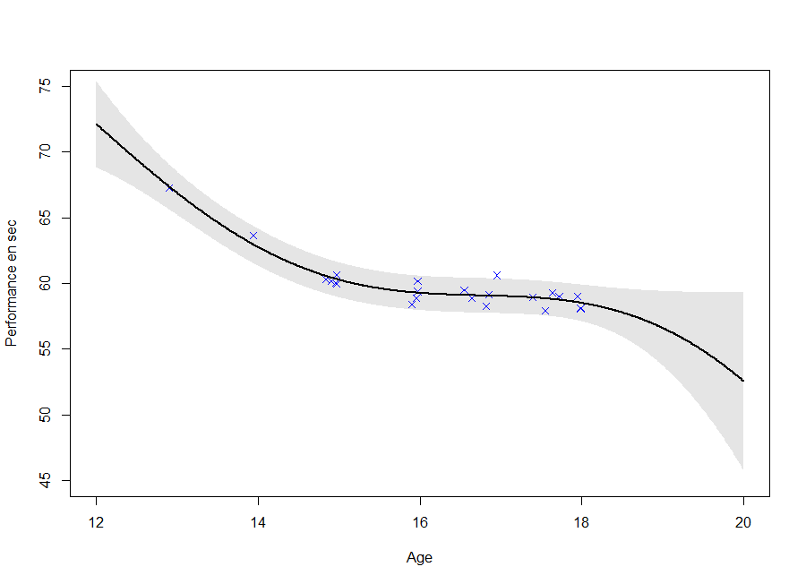
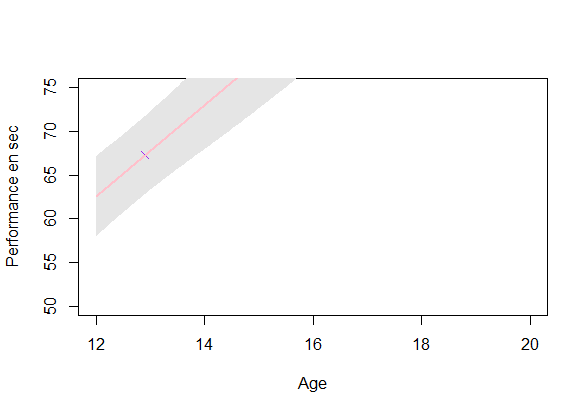
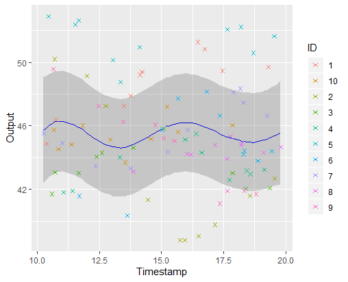
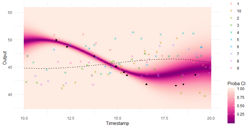
A picture is worth 1000 words

\(\mathbb{E} \left[ \mu_0(\textbf{t}) \vert Data \right] \pm CI_{0.95}\)

Iteration counter : 0

A picture is worth 1000 words

\(\mathbb{E} \left[ \mu_0(\textbf{t}) \vert Data \right] \pm CI_{0.95}\)

Iteration counter : 1

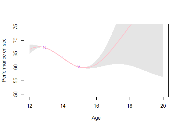
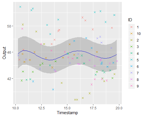
A picture is worth 1000 words

\(\mathbb{E} \left[ \mu_0(\textbf{t}) \vert Data \right] \pm CI_{0.95}\)

Iteration counter : 2

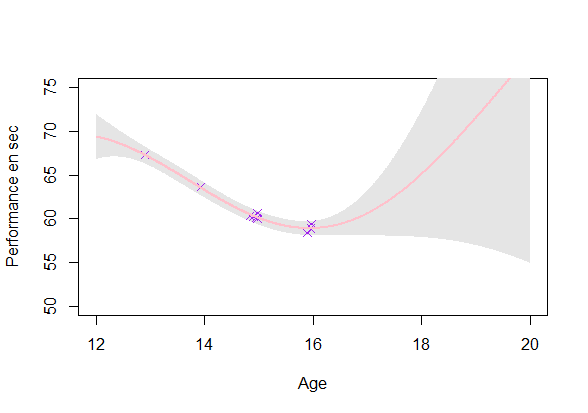
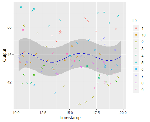
A picture is worth 1000 words

\(\mathbb{E} \left[ \mu_0(\textbf{t}) \vert Data \right] \pm CI_{0.95}\)

Iteration counter : 4

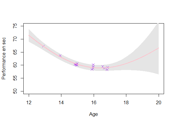
A picture is worth 1000 words

\(\mathbb{E} \left[ \mu_0(\textbf{t}) \vert Data \right] \pm CI_{0.95}\)

Iteration counter : 6 \(\rightarrow\) break and return

Making predictions

\[ \forall i, \ \ y_i(t) = \mu_0(t) + f_i(t) + \epsilon_i \]

Suppose that, after the learning step, you observe some data \(y_*(\textbf{t}_*)\) from a new individual, and want to make predictions at timestamps \(\textbf{t}^p\).

Multi-task learning consists in improving performance by sharing information across individuals.

Without external information:

\(p(\begin{bmatrix} y_*^{\textbf{t}_*} \\ y_*^{\textbf{t}_p} \\ \end{bmatrix}) = \mathcal{N}( \begin{bmatrix} \mu_0^{\textbf{t}_*} \\ \mu_0^{\textbf{t}^p} \\ \end{bmatrix}, \begin{pmatrix} \Psi_*^{\textbf{t}_*,\textbf{t}_*} & \Psi_*^{\textbf{t}_*,\textbf{t}^p} \\ \Psi_*^{\textbf{t}^p,\textbf{t}_*} & \Psi_*^{\textbf{t}^p,\textbf{t}^p} \end{pmatrix})\)

Making predictions: the key idea

Multi-task regression : conditioning on other observations Incertitude on the mean process : integrate over \(\mu_0\)

\[\begin{align} p(y_* \vert \textbf{y}) &= \int p(y_*, \mu_0 \vert \textbf{y}) \ d \mu_0\\ &\underbrace{=}_{Bayes} \int p(y_* \vert \textbf{y}, \mu_0) p(\mu_0 \vert \textbf{y}) \ d \mu_0 \\ &\underbrace{=}_{(y_i \vert \mu_0)_i \perp \!\!\! \perp} \int p(y_* \vert \mu_0) p(\mu_0 \vert \textbf{y}) \ d \mu_0 \\ &= \int \mathcal{N}(y_*; \mu_0, \Psi_*) \mathcal{N}(\mu_0; \hat{m}_0, \hat{K}) \ d \mu_0 \\ &= \mathcal{N}( \hat{m}_0, \Gamma_* = \Psi_* + \hat{K}) \end{align}\]

Making predictions: additional steps

• \(\hat{\theta}_*, \hat{\sigma}_*^2 = \underset{\theta_*, \sigma_*^2}{\arg\max} \ \mathbb{E}_{\mu_0} [ \log \ p(\textbf{y}_*(\textbf{t}_*), \mu_0(\textbf{t}_*) \vert \theta_*, \sigma_*^2 )]\)

• Prior: \(p(\begin{bmatrix} y_*^{\textbf{t}_*} \\ y_*^{\textbf{t}_p} \\ \end{bmatrix} \vert \textbf{y}) = \mathcal{N}( \begin{bmatrix} \hat{m}_0^{\textbf{t}_*} \\ \hat{m}_0^{\textbf{t}_p} \\ \end{bmatrix}, \begin{pmatrix} \Gamma_{**} & \Gamma_{*p} \\ \Gamma_{p*} & \Gamma_{pp} \end{pmatrix})\)

• Posterior: \(p(y_*^{\textbf{t}^p} \vert y_*^{\textbf{t}_*}, \textbf{y}) = \mathcal{N} \Big( \hat{\mu}_{*}^{\textbf{t}^p} , \hat{\Gamma}_{*}^{\textbf{t}^p} \Big)\)

with:

• \(\hat{\mu}_{*}^{\textbf{t}^p} = \hat{m}_0^{\textbf{t}_p} + \Gamma_{p*}\Gamma_{**}^{-1} (y_*^{\textbf{t}_*} - \hat{m}_0^{\textbf{t}_*})\)
• \(\hat{\Gamma}_{*}^{\textbf{t}^p} = \Gamma_{pp} - \Gamma_{p*}\Gamma_{**}^{-1} \Gamma_{*p}\)

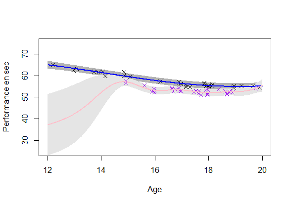
A GIF is worth \(10^9\) words

• Same data, same hyperparameters from learning
• Standard GP (left) | MAGMA (right)

A GIF is worth \(10^9\) words

We talked about clustering, did we ?

A unique underlying mean process might be insufficient

\(\rightarrow\) Mixture model of multitask GP:

\[\forall i , \forall k , \ \ y_i(t) \vert (Z_{ik} = 1) = \mu_k(t) + f_i(t) + \epsilon_i\] with:

• \(Z_{i} \sim \mathcal{M}(1, \boldsymbol{\pi} = (\pi_1, \dots, \pi_K)), \ Z_i \perp \!\!\! \perp\)
• \(\mu_k(\cdot) \sim \mathcal{GP}(m_k(\cdot), C_{\gamma_k}(\cdot,\cdot)), \ \mu_k \perp \!\!\! \perp\)
• \(f_i(\cdot) \sim \mathcal{GP}(0, \Sigma_{\theta_i}(\cdot,\cdot)), \ f_i \perp \!\!\! \perp\)
• \(\epsilon_i \sim \mathcal{N}(0, \sigma_i^2), \ \epsilon_i \perp \!\!\! \perp\)

It follows that:

\[y_i(\cdot) \vert \{ (\mu_k)_k, \boldsymbol{\pi} \} \sim \sum\limits_{k=1}^K{\pi_k \ \mathcal{GP}\Big(\mu_k(\cdot), \Psi_i(\cdot, \cdot) \Big)}\]

Learning

We need to learn the following quantities:

• \(p((\mu_k)_k \vert \textbf{y})\), mean processes' hyper-posteriors
• \(p((Z_i)_i \vert \textbf{y})\), clustering variables' hyper-posteriors
• \(\Theta = \{ (\gamma_k)_k, (\theta_i)_i, (\sigma_i^2), \boldsymbol{\pi} \}\), the hyper-parameters

Unfortunately \((\mu_k)_k\) and \((Z_i)_i\) are posterior dependent

\(\rightarrow\) Variational inference, to maintain closed-form approximations. For any distribution \(q\):

\(\log p(\textbf{y} \vert \Theta) = \mathcal{L}(q; \Theta) + KL \big( q \vert \vert p(\boldsymbol{\mu}, \boldsymbol{Z} \vert \textbf{y}, \Theta)\big)\)

Approximation assumption: \(q(\boldsymbol{\mu}, \boldsymbol{Z}) = q_{\boldsymbol{\mu}}(\boldsymbol{\mu})q_{\boldsymbol{Z}}(\boldsymbol{Z})\)

\(\rightarrow\) \(\mathcal{L}(q; \Theta)\) provides a lower bound to maximize

Variational EM

Step E: Optimize \(\mathcal{L}(q; \Theta)\) w.r.t. \(q\)

• \(\hat{q}_{\boldsymbol{Z}}(\boldsymbol{Z}) = \prod\limits_{i = 1}^M \mathcal{M}(Z_i;1, \boldsymbol{\tau}_i)\)

• \(\hat{q}_{\boldsymbol{\mu}}(\boldsymbol{\mu}) = \prod\limits_{k = 1}^K \mathcal{N}(\mu_k;\hat{m}_k, \hat{C}_k)\)

Step M: Optimize \(\mathcal{L}(q; \Theta)\) w.r.t. \(\Theta\)

• \(\hat{\Theta} = \text{arg}\max\limits_{\Theta} \mathbb{E}_{\boldsymbol{\mu},\boldsymbol{Z}} \left[ \log p(\textbf{y},\boldsymbol{\mu}, \boldsymbol{Z} \vert \Theta)\right]\)

\(\rightarrow\) Iterate on these steps until convergence

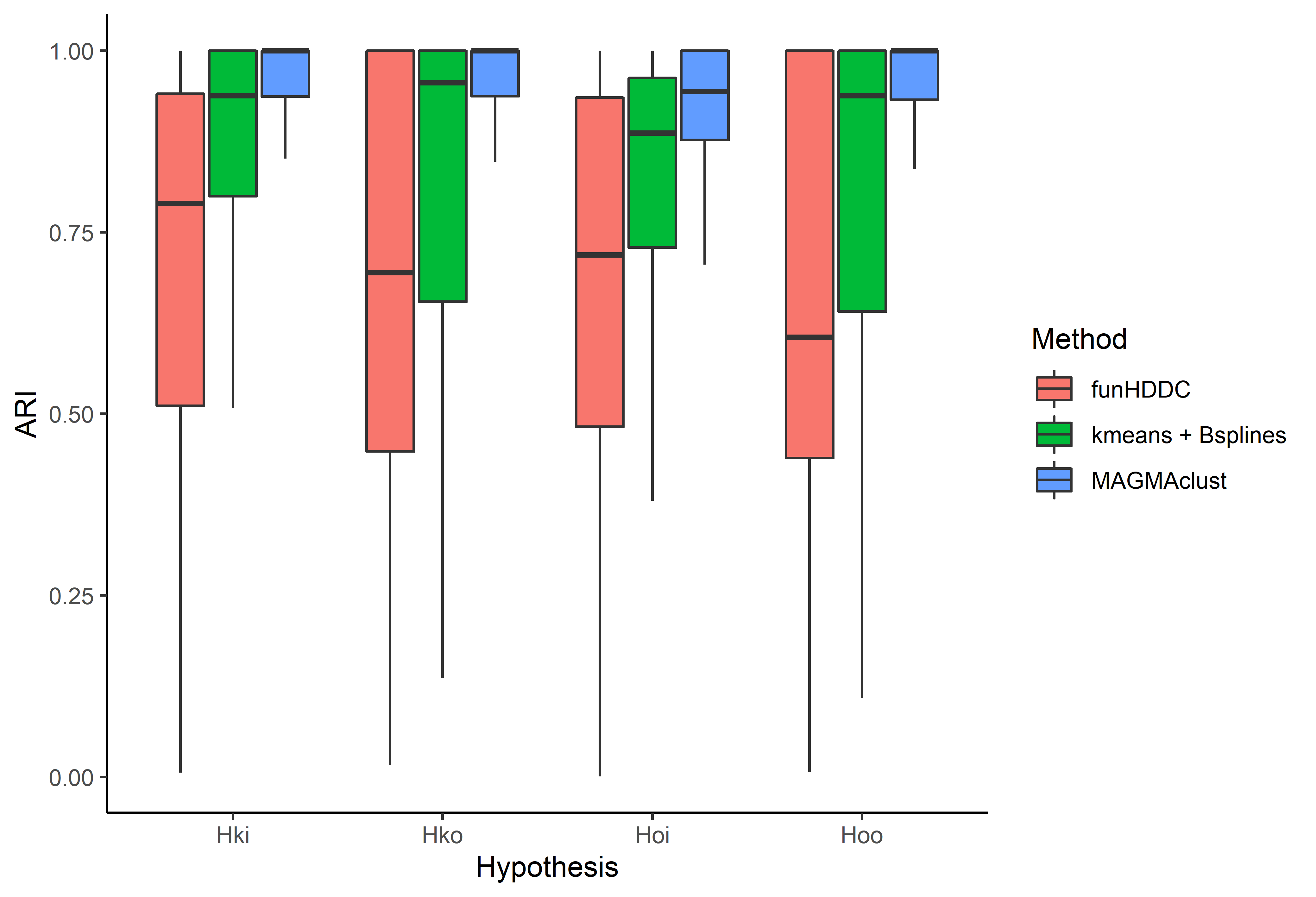
4 different model assumptions

• \(\mathcal{H}_{oo}: \gamma_0 = \gamma_k, \theta_0 = \theta_i, \sigma_0^2 = \sigma_i^2, \ \forall i, \forall k\)
• \(\mathcal{H}_{ko}: \gamma_k \neq \gamma_l, \theta_0 = \theta_i, \sigma_0^2 = \sigma_i^2, \ \forall i, \forall k,l\)
• \(\mathcal{H}_{oi}: \gamma_0 = \gamma_k, \theta_i \neq \theta_j, \sigma_i^2 \neq \sigma_j^2, \ \forall i,j, \forall k\)
• \(\mathcal{H}_{ki}: \gamma_0 \neq \gamma_k, \theta_0 \neq \theta_i, \sigma_0^2 \neq \sigma_i^2, \ \forall i,j, \forall k,l\)

\(\rightarrow\) Allows a multi-task aspect on the covariance structure, and a compromise between number of hyper-parameters and flexibility:

• \(\mathcal{H}_{oo}\): 3 hyper-parameters
• \(\mathcal{H}_{ko}\): K + 2 hyper-parameters
• \(\mathcal{H}_{oa}\): 2M + 1 hyper-parameters
• \(\mathcal{H}_{ki}\): 2M + K hyper-parameters

Prediction

• EM for estimating \(Z_*, \theta_*,\) and \(\sigma_*^2\)

• Multi-task prior: \(p(\begin{bmatrix} y_*^{\textbf{t}_*} \\ y_*^{\textbf{t}_p} \\ \end{bmatrix} \vert Z_{*k}=1 , \textbf{y}) = \mathcal{N}( \begin{bmatrix} \hat{m}_k^{\textbf{t}_*} \\ \hat{m}_k^{\textbf{t}_p} \\ \end{bmatrix}, \begin{pmatrix} \Gamma_{**}^k & \Gamma_{*p}^k \\ \Gamma_{p*}^k & \Gamma_{pp}^k \end{pmatrix}), \forall k\)

• Multi-task posterior: \(p(y_*^{\textbf{t}^p} \vert y_*^{\textbf{t}_*}, Z_{*k} = 1, \textbf{y}) = \mathcal{N} \big( \hat{\mu}_{*k}^{\textbf{t}^p} , \hat{\Gamma}_{*k}^{\textbf{t}^p} \big), \ \forall k\)

• Predictive multi-task GPs mixture: \(p(y_*^{\textbf{t}^p} \vert y_*^{\textbf{t}_*}, \textbf{y}) = \sum\limits_{k = 1}^{K} \tau_{*k} \ \mathcal{N} \big( \hat{\mu}_{*k}^{\textbf{t}^p} , \hat{\Gamma}_{*k}^{\textbf{t}^p} \big)\)

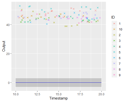
Illustration: GP regression

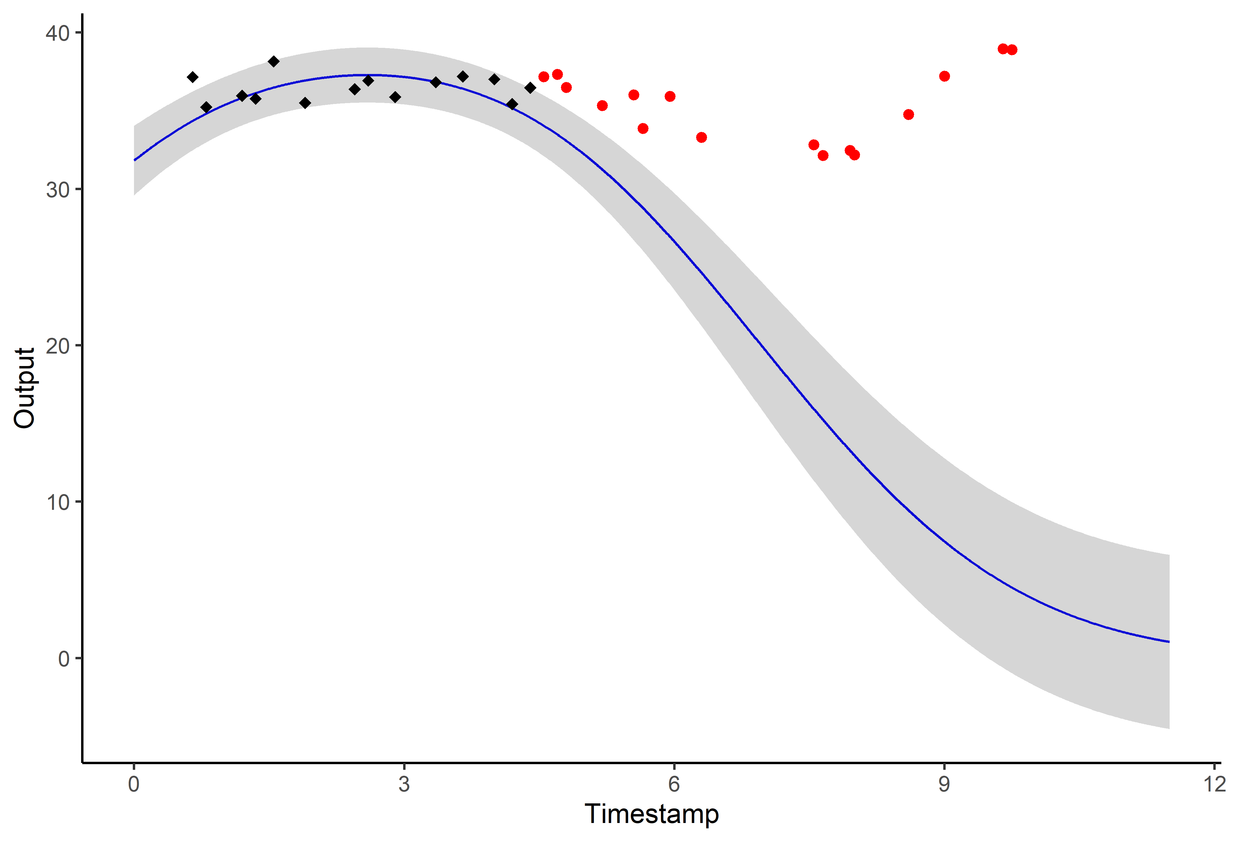
Illustration: MAGMA

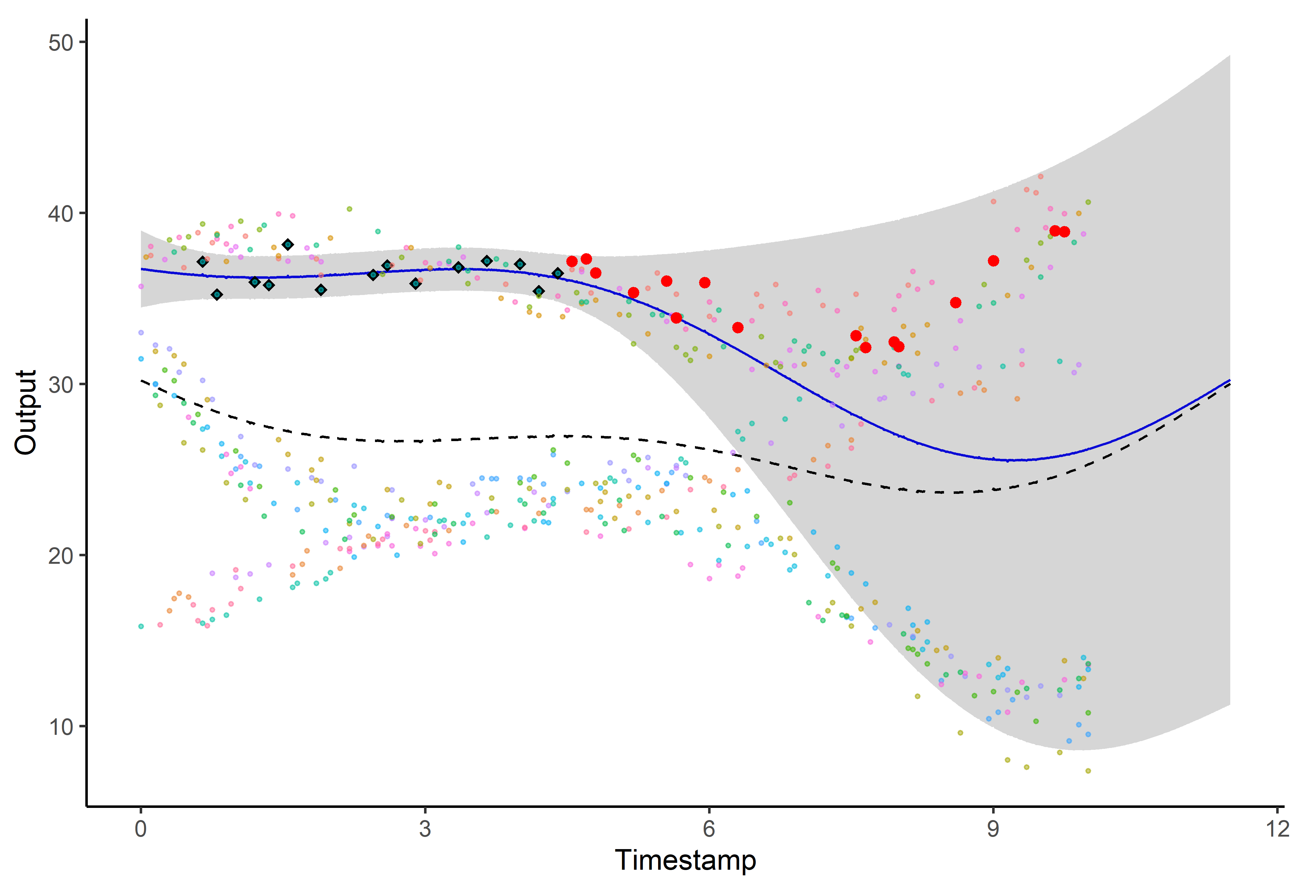
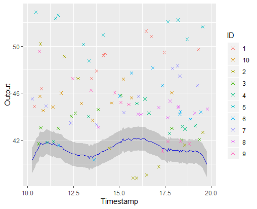
Illustration: MAGMAclust

Illustration: MAGMAclust

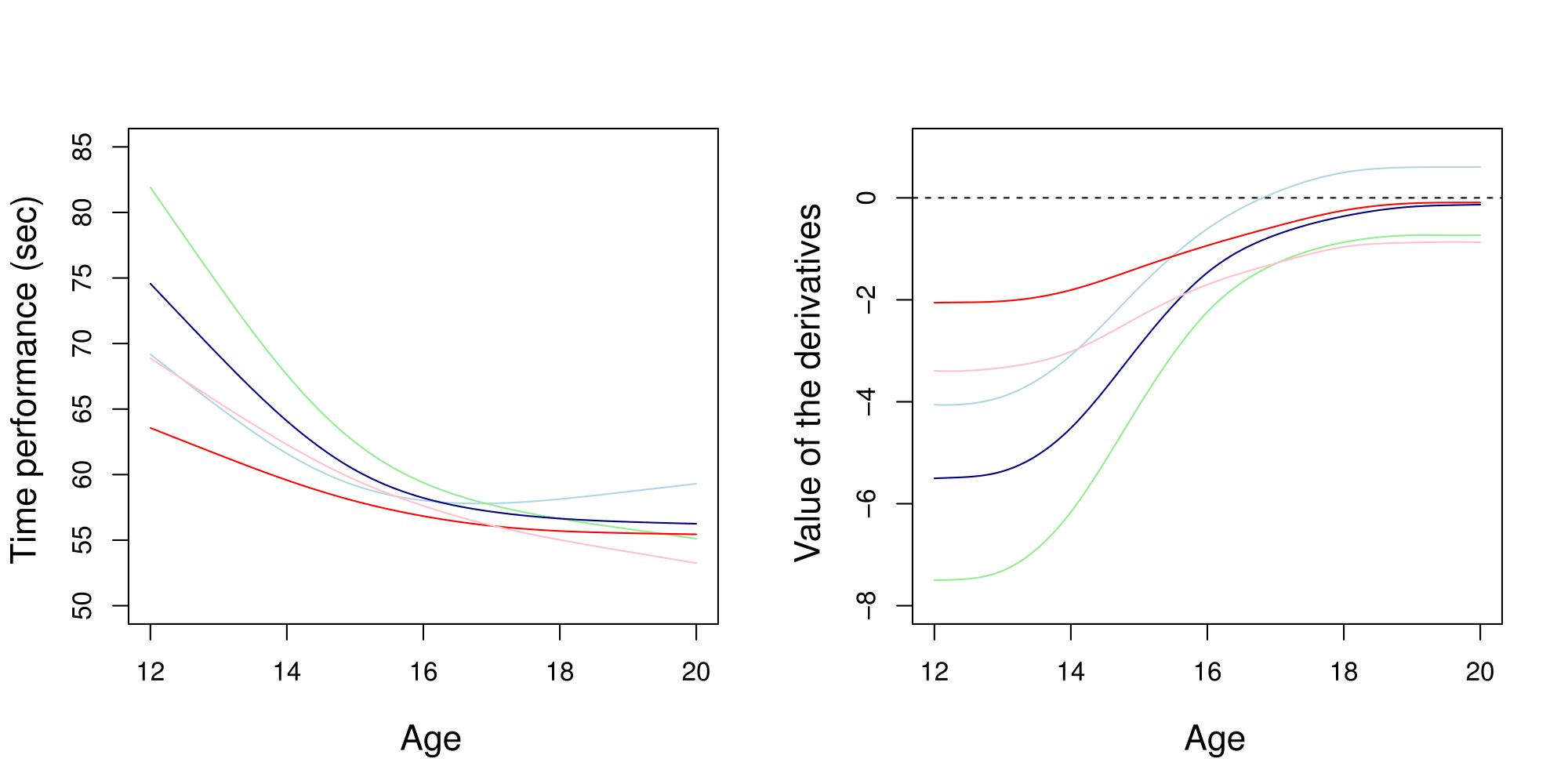
Estimation of the mean processes

Clustering performances

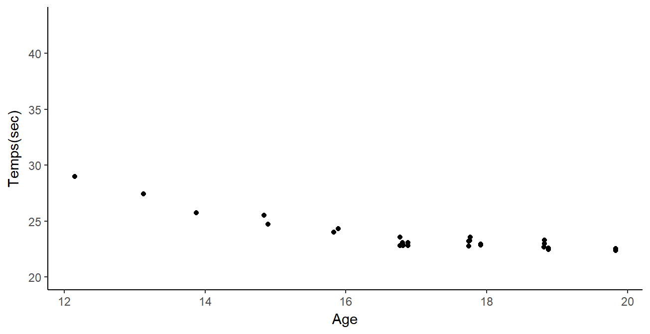
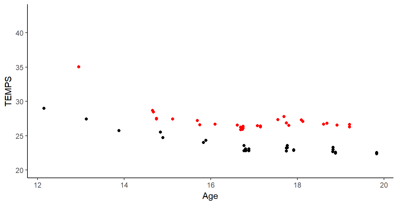
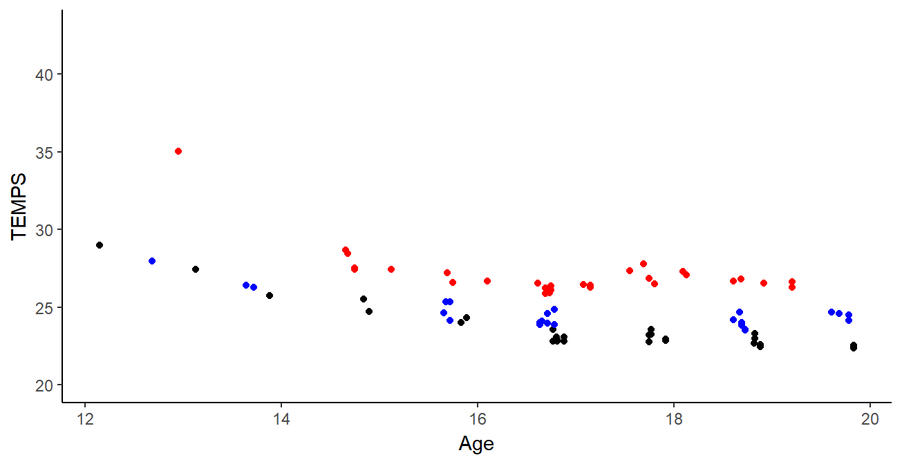
And what about the swimmers ?

Did I mention that I like GIFs ?

Why probabilistic predictions matter ?

Making a prediction is \(\mathbb{P}(\)saying something wrong\() \simeq 1\).
A probabilistic prediction tells you how much:

Perspectives

• Enable association with sparse GP approximations

• Extend to multivariate functional regression

• Work on an online version

• Develop a more sophisticated model selection tool

• Integrate to the app and launch tests with FFN

• Listen to new good ideas that you are about to give me

References

A cat GIF is priceless

References

Pattern Recognition and Machine Learning - Bishop - 2006
Gaussian processes for machine learning - Rasmussen & Williams - 2006
Curve prediction and clustering with mixtures of Gaussian process [...] - Shi & Wang - 2008
Gaussian Process Regression Analysis for Functional Data - Shi & Choi - 2011
Career Performance Trajectories in Track and Field Jumping Events [...] - Boccia & al - 2017
Efficient Bayesian hierarchical functional data analysis [...] - Yang & al - 2017
Excelling at youth level in competitive track and field [...] - Kearney & Hayes - 2018
Functional Data Analysis in Sport Science: Example of Swimmers' [...] - Leroy & al. - 2018
MAGMA: Inference and Prediction with Multi-Task Gaussian Processes - Leroy & al. - preprint Cluster-Specific Predictions with Multi-Task Gaussian Processes - Leroy & al. - preprint