![image alt <]()
![image alt >]()
Mélange de processus gaussiens multi-tâches et prédictions cluster-spécifiques
Arthur Leroy - MAP5, Université de Paris
en collaboration avec
- Servane Gey - MAP5, Université de Paris
- Benjamin Guedj - Inria - University College London
- Pierre Latouche - MAP5, Université de Paris
52èmes Journées de Statistiques - Nice (ou presque) - 07/06/2021
Context
\[y_i = \color{red}{f}(x_i) + \epsilon\]
Context
\[y_i^{\color{green}{k}} = \color{red}{f}(x_i^{\color{green}{k}}) + \epsilon\]
- Training: learn \(\color{red}{f}\), and create \(\color{green}{K}\) groups from a training dataset \(\{ (x_1, y_1), \dots, (x_M, y_M) \}\),
- Prediction: for a new input \(x_*\), simultaneously compute membership probabilities for each group \(\tau_*^\color{green}{k}\) and cluster specific probabilistic predictions for the output \(p(y_*^{\color{green}{k}})\).

Gaussian process regression
No restrictions on \(\color{red}{f}\) but a prior distribution on a functional space: \(\color{red}{f} \sim \mathcal{GP}(0,C(\cdot,\cdot))\)

- Powerful non parametric method offering probabilistic predictions,
- Computational complexity in \(\mathcal{O}(N^3)\), with N the number of observations,
- Correspondence with infinitly wide (deep) neural networks (Neal - 1994, Lee et al. - 2018).
Modelling and prediction with a unique GP

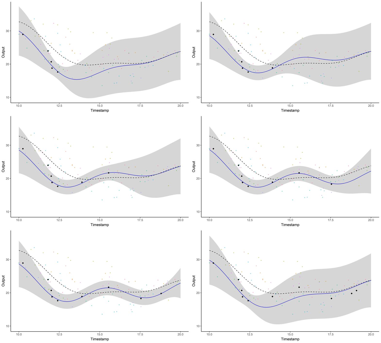
GPs are great for modelling time series although insufficient for long-term predictions.
Multi-task GP with common mean (Magma)
\[y_i = \mu_0 + f_i + \epsilon_i\]
with:
- \(\mu_0 \sim \mathcal{GP}(m_0, K_{\theta_0}),\)
- \(f_i \sim \mathcal{GP}(0, \Sigma_{\theta_i}), \ \perp \!\!\! \perp_i,\)
- \(\epsilon_i \sim \mathcal{GP}(0, \sigma_i^2), \ \perp \!\!\! \perp_i.\)
It follows that:
\[y_i \mid \mu_0 \sim \mathcal{GP}(\mu_0, \Sigma_{\theta_i} + \sigma_i^2 I), \ \perp \!\!\! \perp_i\]
\(\rightarrow\) Unified GP framework with a common mean process \(\mu_0\), and individual-specific process \(f_i\),
\(\rightarrow\) Naturaly handles irregular grids of input data.
Hyper-parameters and \(\mu_0\)’s hyper-posterior are learned thanks to an EM algorithm.
Prediction
For a new individual, we observe some data \(y_*(\textbf{t}_*)\). Let us recall:
\[y_* \mid \mu_0 \sim \mathcal{GP}(\mu_0, \boldsymbol{\Psi}_{\theta_*, \sigma_*^2}), \ \perp \!\!\! \perp_i\]
Goals:
- derive a analytical predictive distribution at arbitrary inputs \(\mathbf{t}^{p}\),
- sharing the information from training individuals, stored in the mean process \(\mu_0\).
Difficulties:
- the model is conditionned over \(\mu_0\), a latent, unobserved quantity,
- defining the adequate target distribution is not straightforward,
- working on a new grid of inputs \(\mathbf{t}^{p}_{*}= (\mathbf{t}_{*}, \mathbf{t}^{p})^{\intercal},\) potentially distinct from \(\mathbf{t}.\)
Prediction: the key idea
Defining a multi-task prior distribution by:
- conditioning on training data,
- integrating over \(\mu_0\)’s hyper-posterior distribution.
\[\begin{align} p(y_* (\textbf{t}_*^{p}) \mid \textbf{y}) &= \int p\left(y_* (\textbf{t}_*^{p}) \mid \textbf{y}, \mu_0(\textbf{t}_*^{p})\right) p(\mu_0 (\textbf{t}_*^{p}) \mid \textbf{y}) \ d \mu_0(\mathbf{t}^{p}_{*}) \\ &= \int \underbrace{ p \left(y_* (\textbf{t}_*^{p}) \mid \mu_0 (\textbf{t}_*^{p}) \right)}_{\mathcal{N}(y_*; \mu_0, \Psi_*)} \ \underbrace{p(\mu_0 (\textbf{t}_*^{p}) \mid \textbf{y})}_{\mathcal{N}(\mu_0; \hat{m}_0, \hat{K})} \ d \mu_0(\mathbf{t}^{p}_{*}) \\ &= \mathcal{N}( \hat{m}_0 (\mathbf{t}^{p}_{*}), \Gamma) \end{align}\]
A GIF is worth a thousand words

Magma + Clustering = MagmaClust
A unique underlying mean process might be too restrictive.
\(\rightarrow\) Mixture of multi-task GPs:
\[y_i = \mu_0 + f_i + \epsilon_i\]
with:
- \(\color{green}{Z_{i}} \sim \mathcal{M}(1, \color{green}{\boldsymbol{\pi}}), \ \perp \!\!\! \perp_i,\)
- \(\mu_0 \sim \mathcal{GP}(m_0, K_{\theta_0}), \ \perp \!\!\! \perp_k,\)
- \(f_i \sim \mathcal{GP}(0, \Sigma_{\theta_i}), \ \perp \!\!\! \perp_i,\)
- \(\epsilon_i \sim \mathcal{GP}(0, \sigma_i^2), \ \perp \!\!\! \perp_i.\)
It follows that:
\[y_i \mid \mu_0 \sim \mathcal{GP}(\mu_0, \Psi_i), \ \perp \!\!\! \perp_i\]
Magma + Clustering = MagmaClust
A unique underlying mean process might be too restrictive.
\(\rightarrow\) Mixture of multi-task GPs:
\[y_i \mid \{\color{green}{Z_{ik}} = 1 \} = \mu_{\color{green}{k}} + f_i + \epsilon_i\]
with:
- \(\color{green}{Z_{i}} \sim \mathcal{M}(1, \color{green}{\boldsymbol{\pi}}), \ \perp \!\!\! \perp_i,\)
- \(\mu_{\color{green}{k}} \sim \mathcal{GP}(m_{\color{green}{k}}, \color{green}{C_{\gamma_{k}}})\ \perp \!\!\! \perp_{\color{green}{k}},\)
- \(f_i \sim \mathcal{GP}(0, \Sigma_{\theta_i}), \ \perp \!\!\! \perp_i,\)
- \(\epsilon_i \sim \mathcal{GP}(0, \sigma_i^2), \ \perp \!\!\! \perp_i.\)
It follows that:
\[y_i \mid \{ \boldsymbol{\mu} , \color{green}{\boldsymbol{\pi}} \} \sim \sum\limits_{k=1}^K{ \color{green}{\pi_k} \ \mathcal{GP}\Big(\mu_{\color{green}{k}}, \Psi_i^\color{green}{k} \Big)}, \ \perp \!\!\! \perp_i\]
Learning
The integrated likelihood is not tractable anymore due to posterior dependencies between \( \boldsymbol{\mu} = \{\mu_\color{green}{k}\}_\color{green}{k}\) and \(\mathbf{Z}= \{Z_i\}_i\).
Variational inference still allows us to maintain closed-form approximations. For any distribution \(q\):
\[\log p(\textbf{y} \mid \Theta) = \mathcal{L}(q; \Theta) + KL \big( q \mid \mid p(\boldsymbol{\mu}, \boldsymbol{Z} \mid \textbf{y}, \Theta)\big)\]
The posterior independance is forced by an approximation assumption:
\[q(\boldsymbol{\mu}, \boldsymbol{Z}) = q_{\boldsymbol{\mu}}(\boldsymbol{\mu})q_{\boldsymbol{Z}}(\boldsymbol{Z}).\]
Maximising the lower bound \(\mathcal{L}(q; \Theta)\) induces natural factorisations over clusters and individuals for the variational distributions.
Variational EM: E step
The optimal variational distributions are analytical and factorise such as:
\[ \begin{align} \hat{q}_{\boldsymbol{\mu}}(\boldsymbol{\mu}) &= \color{green}{\prod\limits_{k = 1}^K} \mathcal{N}(\mu_\color{green}{k};\hat{m}_\color{green}{k}, \hat{\textbf{C}}_\color{green}{k}) \\ \hat{q}_{\boldsymbol{Z}}(\boldsymbol{Z}) &= \prod\limits_{i = 1}^M \mathcal{M}(Z_i;1, \color{green}{\boldsymbol{\tau}_i}) \end{align} \]
with:
Variational EM: M step
Optimising \(\mathcal{L}(\hat{q}; \Theta)\) w.r.t. \(\Theta\) induces independant maximisation problems:
\[ \begin{align*} \hat{\Theta} &= \text{arg}\max\limits_{\Theta} \mathbb{E}_{\boldsymbol{\mu},\boldsymbol{Z}} \left[ \log p(\textbf{y},\boldsymbol{\mu}, \boldsymbol{Z} \mid \Theta)\right] \\ &= \sum\limits_{k = 1}^{K}\ \mathcal{N} \left( \hat{m}_k; \ m_k, \boldsymbol{C}_{\color{green}{\gamma_k}} \right) - \dfrac{1}{2} \textrm{tr}\left( \mathbf{\hat{C}}_k\boldsymbol{C}_{\color{green}{\gamma_k}}^{-1}\right) \\ & \hspace{1cm} + \sum\limits_{k = 1}^{K}\sum\limits_{i = 1}^{M}\tau_{ik}\ \mathcal{N} \left( \mathbf{y}_i; \ \hat{m}_k, \boldsymbol{\Psi}_{\color{brown}{\theta_i}, \color{brown}{\sigma_i^2}} \right) - \dfrac{1}{2} \textrm{tr}\left( \mathbf{\hat{C}}_k\boldsymbol{\Psi}_{\color{brown}{\theta_i}, \color{brown}{\sigma_i^2}}^{-1}\right) \\ & \hspace{1cm} + \sum\limits_{k = 1}^{K}\sum\limits_{i = 1}^{M}\tau_{ik}\log \color{green}{\pi_{k}} \end{align*} \]
Prediction
- EM for estimating \(p(\color{green}{Z_*} \mid \textbf{y}, \hat{\Theta})\), \(\hat{\theta}_*\) and \(\hat{\sigma}_*^2\),
-
Multi-task prior for each cluster:
\[p \left( \begin{bmatrix} y_*(\color{red}{\mathbf{t}_{*}}) \\ y_*(\color{blue}{\mathbf{t}^{p}}) \\ \end{bmatrix} \mid \color{green}{Z_{*k}} = 1, \textbf{y} \right) = \mathcal{N} \left( \begin{bmatrix} y_*(\color{red}{\mathbf{t}_{*}}) \\ y_*(\color{blue}{\mathbf{t}^{p}}) \\ \end{bmatrix}; \ \begin{bmatrix} \hat{m}_\color{green}{k}(\color{red}{\mathbf{t}_{*}}) \\ \hat{m}_\color{green}{k}(\color{blue}{\mathbf{t}^{p}}) \\ \end{bmatrix}, \begin{pmatrix} \Gamma_{\color{red}{**}}^\color{green}{k} & \Gamma_{\color{red}{*}\color{blue}{p}}^\color{green}{k} \\ \Gamma_{\color{blue}{p}\color{red}{*}}^\color{green}{k} & \Gamma_{\color{blue}{pp}}^\color{green}{k} \end{pmatrix} \right), \forall \color{green}{k},\]
-
Multi-task posterior for each cluster:
\[ p(y_*(\color{blue}{\mathbf{t}^{p}}) \mid \color{green}{Z_{*k}} = 1, y_*(\color{red}{\mathbf{t}_{*}}), \textbf{y}) = \mathcal{N} \Big( y_*(\color{blue}{\mathbf{t}^{p}}); \ \hat{\mu}_{*}^\color{green}{k}(\color{blue}{\mathbf{t}^{p}}) , \hat{\Gamma}_{\color{blue}{pp}}^\color{green}{k} \Big), \forall \color{green}{k}, \]
\(\hat{\mu}_{*}^\color{green}{k}(\color{blue}{\mathbf{t}^{p}}) = \hat{m}_\color{green}{k}(\color{blue}{\mathbf{t}^{p}}) + \Gamma^\color{green}{k}_{\color{blue}{p}\color{red}{*}} {\Gamma^\color{green}{k}_{\color{red}{**}}}^{-1} (y_*(\color{red}{\mathbf{t}_{*}}) - \hat{m}_\color{green}{k} (\color{red}{\mathbf{t}_{*}}))\)
\(\hat{\Gamma}_{\color{blue}{pp}}^\color{green}{k} = \Gamma_{\color{blue}{pp}}^\color{green}{k} - \Gamma_{\color{blue}{p}\color{red}{*}}^\color{green}{k} {\Gamma^{\color{green}{k}}_{\color{red}{**}}}^{-1} \Gamma^{\color{green}{k}}_{\color{red}{*}\color{blue}{p}}\) -
Predictive multi-task GPs mixture:
\[p(y_*(\color{blue}{\textbf{t}^p}) \mid y_*(\color{red}{\textbf{t}_*}), \textbf{y}) = \color{green}{\sum\limits_{k = 1}^{K} \tau_{*k}} \ \mathcal{N} \big( y_*(\color{blue}{\mathbf{t}^{p}}); \ \hat{\mu}_{*}^\color{green}{k}(\textbf{t}^p) , \hat{\Gamma}_{pp}^\color{green}{k}(\textbf{t}^p) \big).\]
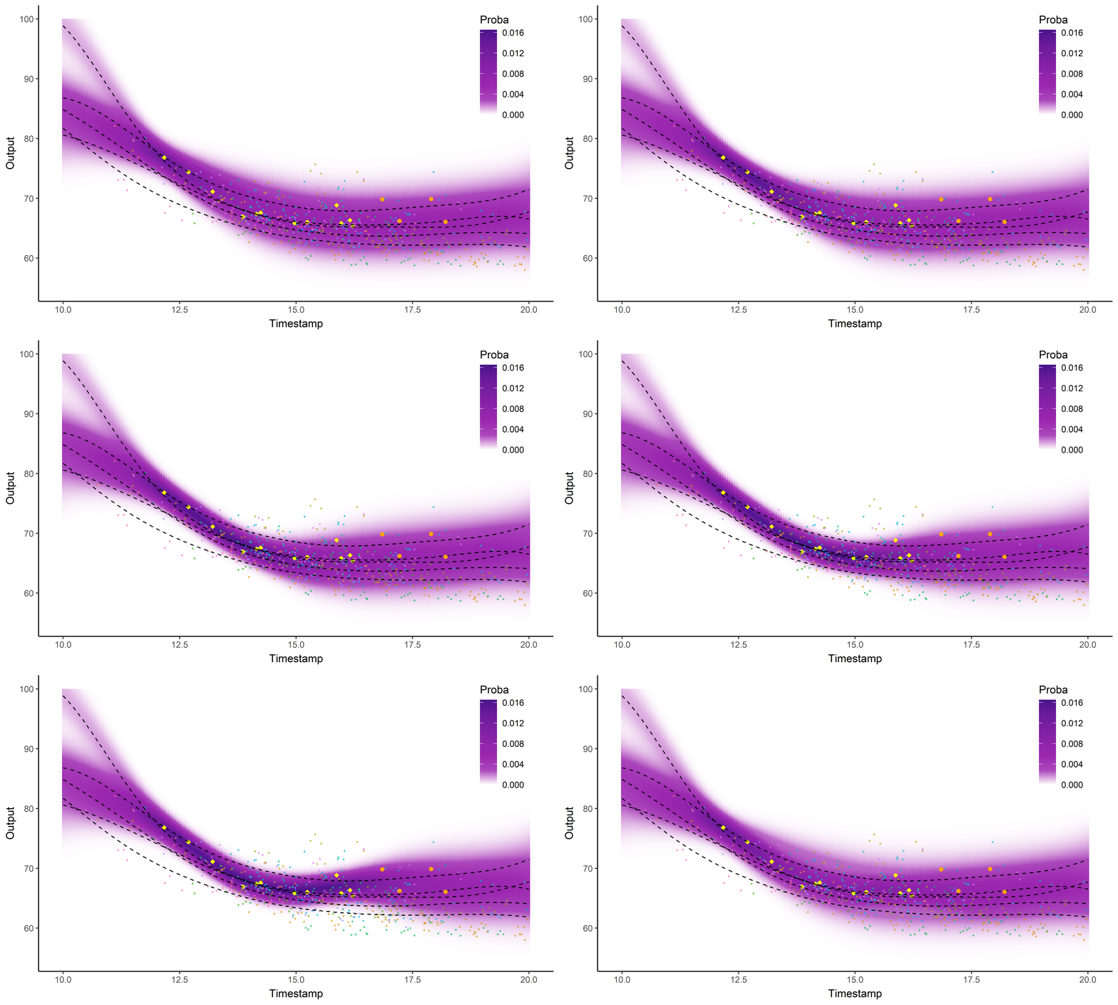
Illustration: Magma vs MagmaClust


Clustering and prediction performances


Application to prediction of swimming performance curves

Application to prediction of swimming performance curves

Application to prediction of swimming performance curves

Predictive performances on swimmers datasets

Did I mention that I like GIFs ?

Perspectives
-
Enable association with sparse GP approximations, -
Extend to multivariate functional regression, -
Develop an online version.
-
Neal - Priors for infinite networks - University of Toronto - 1994
-
Lee et al. - Deep Neural Networks as Gaussian Processes - ICLR - 2018
-
Leroy et al. - Magma: Inference and Prediction with Multi-Task Gaussian Processes - Under review - 2020
- Leroy et al. - Cluster-Specific Predictions with Multi-Task Gaussian Processes - Under review - 2020
Model selection in MagmaClust
After convergence of the VEM algorithm, a variational-BIC expression can be derived as:
\[\begin{align*} V_{BIC} &= \mathcal{L}(\hat{q}; \hat{\Theta}) - \dfrac{\mathrm{card}\{HP \}}{2} \log M \\ &= \sum\limits_{i=1}^M \sum\limits_{k=1}^K \left[ \tau_{ik} \left( \log \mathcal{N}\left( \mathbf{y}_i; \hat{m}_k(\mathbf{t}_i), {\boldsymbol{\Psi}_{\hat{\theta}_i, \hat{\sigma}_i^2}^{\mathbf{t}_i}} \right) - \dfrac{1}{2} Tr ( \mathbf{\hat{C}}_k^{\mathbf{t}} {\boldsymbol{\Psi}_{\hat{\theta}_i, \hat{\sigma}_i^2}^{\mathbf{t}_i}}^{-1}) + \log \dfrac{\hat{\pi_k}}{\tau_{ik}} \right) \right] \\ & \hspace{0.5cm} + \sum\limits_{k=1}^K \Bigg[ \log \mathcal{N} \left( \hat{m}_k(\textbf{t}); m_k(\mathbf{t}) , {\mathbf{C}_{\hat{\gamma}_k}^{\mathbf{t}^{p}_{*}}} \right) - \dfrac{1}{2} Tr( \mathbf{\hat{C}}_k^{\mathbf{t}} {\mathbf{C}_{\hat{\gamma}_k}^{\mathbf{t}^{p}_{*}}}^{-1}) \\ & \hspace{2cm} + \dfrac{1}{2} \log \mid \mathbf{\hat{C}}_k^{\mathbf{t}} \mid + N \log 2 \pi + N \Bigg] - \dfrac{\alpha_i + \alpha_k + (K - 1)}{2} \log M. \end{align*}\]
Model selection performances of VBIC

Appendix
Two important prediction steps of Magma have been omitted for clarity:
- Recomputing the hyper-posterior distribution on the new grid: \[ p\left( \mu_0 (\textbf{t}_*^{p}) \mid \textbf{y} \right), \]
- Estimating the hyper-parameters of the new individual: \[ \hat{\theta}_*, \hat{\sigma}_*^2 = \underset{\theta_*, \sigma_*^2}{\arg\max} \ p(y_* (\textbf{t}_*) \mid \textbf{y}, \theta_*, \sigma_*^2 ). \]
The computational complexity for learning is given by:
- Magma: \[ \mathcal{O}(M\times N_i^3 + N^3) \]
- MagmaClust: \[ \mathcal{O}(M\times N_i^3 + K \times N^3) \]
Appendix: MagmaClust, remaining clusters


