---

Multi-Means Gaussian Processes: A novel probabilistic framework for multi-correlated longitudinal data

---

Context

Gaussian processes are elegant and well-suited tools for modelling longitudinal data. Nowadays, it is generally straightforward to:

• Fit a GP on functional or high frequency data (sparse approximations)
• Handle a few correlated time series (LMC, Multi-Output GPs, …)

However, are we able to deal with millions of correlated time series simultaneously?

For our current project, we observe:

• \(\color{blue}{M} \simeq 300\) individuals,
• with \(\color{red}{P} \simeq 700 000\) gene-related time series each,
• observed over \(N \simeq 10\) timestamps.

Context: illustration

Multi-task GP with common mean (Magma)

with:

\(\mu_0 \sim \mathcal{GP}(m_0, K_{\theta_0}),\) \(f_i \sim \mathcal{GP}(0, \Sigma_{\theta_i}),\) \(\epsilon_i \sim \mathcal{GP}(0, \sigma_i^2), \ \perp \!\!\! \perp_i.\)

It follows that:

\(\rightarrow\) Unified GP framework with a common mean process \(\mu_0\), and individual-specific process \(f_i\),

\(\rightarrow\) Naturaly handles irregular grids of input data.

Hyper-parameters and \(\mu_0\)’s hyper-posterior are learned thanks to an EM algorithm.

A GIF is worth a thousand² words

Sharing information across tasks through a common latent process to provide a well-informed mean function for prediction.

Magma + Clustering = MagmaClust

Leroy et al. - Cluster-Specific Predictions with Multi-Task Gaussian Processes - 2020

A unique underlying mean process might be too restrictive.

\(\rightarrow\) Mixture of multi-task GPs:

with:

• \(\mu_{\color{green}{k}} \sim \mathcal{GP}(m_{\color{green}{k}}, \color{green}{C_{\gamma_{k}}})\ \perp \!\!\! \perp_{\color{green}{k}}, \ \ f_i \sim \mathcal{GP}(0, \Sigma_{\theta_i}), \ \epsilon_i \sim \mathcal{GP}(0, \sigma_i^2), \ \perp \!\!\! \perp_i,\)
• \(\color{green}{Z_{i}} \sim \mathcal{M}(1, \color{green}{\boldsymbol{\pi}}), \ \perp \!\!\! \perp_i.\)

It follows that:

An image is still worth many words

Implemented as an R package MagmaClustR: https://github.com/ArthurLeroy/MagmaClustR

Multi-Means Gaussian processes

Different sources of correlation might exist in the data (e.g. multiple genes and individuals)

with:

• \(\mu_{0} \sim \mathcal{GP}(m_{0}, {C_{\gamma_{0}}}), \ f_{\color{blue}{i}} \sim \mathcal{GP}(0, \Sigma_{\theta_{\color{blue}{i}}}), \ \epsilon_{\color{blue}{i}\color{red}{j}} \sim \mathcal{GP}(0, \sigma_{\color{blue}{i}\color{red}{j}}^2), \ \perp \!\!\! \perp_i\)
• \(g_{\color{red}{j}} \sim \mathcal{GP}(0, \Sigma_{\theta_{\color{red}{j}}})\)

Key idea for training: define \(\color{blue}{M}+\color{red}{P} + 1\) different hyper-posterior distributions for \(\mu_0\) by conditioning over the adequate sub-sample of data.

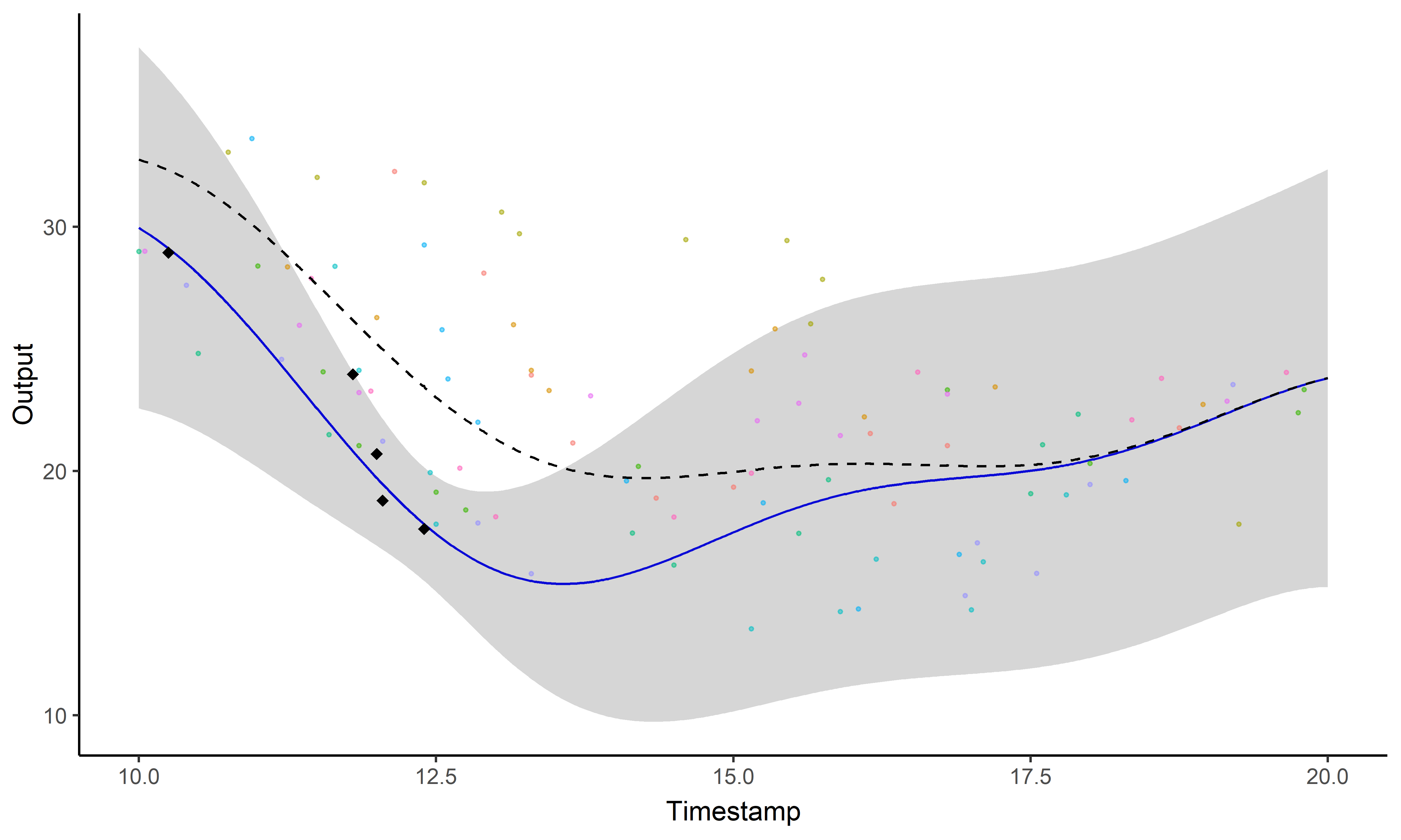
Multi-Means GPs: an adaptive prediction

Multi-Means GPs: an adaptive prediction

Answer to the \(\mathbb{P}(\)first question\() \approx 1\)

\(\rightarrow\) All methods scale linearly with the number of tasks.

\(\rightarrow\) Parallel computing can be used to speed up training.

Overall, the computational complexity is:

• Magma: \[ \mathcal{O}(M\times N_i^3 + N^3) \]
• MagmaClust: \[ \mathcal{O}(M\times N_i^3 + K \times N^3) \]
• Multi-Means Gaussian Processes: \[ \mathcal{O}(M \times P \times N_{ij}^3 + (M + P) \times N^3) \]

Appendix: Clustering and prediction performances

Appendix: MagmaClust, remaining clusters